Anomaly Detection

This notebook shows some basic usage of CapyMOA for anomaly detection tasks.

Algorithms: HalfSpaceTrees, Autoencoder and Online Isolation Forest

Important notes: Prior to version 0.8.2, a lower anomaly score indicated a higher likelihood of an anomaly. This has been updated so that a higher anomaly score now indicates a higher likelihood of an anomaly, aligning with the standard anomaly detection literature.

---

More information about CapyMOA can be found at https://www.capymoa.org.

last update on 28/11/2025

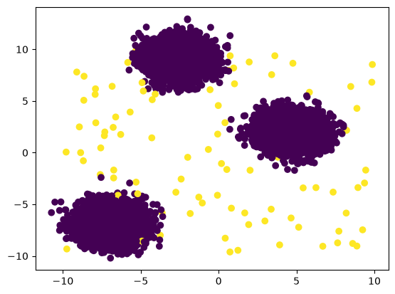
Creating simple anomalous data with sklearn

• Generating a few examples and some simple anomalous data using sklearn.

import matplotlib.pyplot as plt
import numpy as np
from sklearn.datasets import make_blobs

from capymoa.stream import NumpyStream

# generate normal data points
n_samples = 10000
n_features = 2
n_clusters = 3

# generate anomalous data points
n_anomalies = 100  # the anomaly rate is 1%

X, y = make_blobs(
    n_samples=n_samples, n_features=n_features, centers=n_clusters, random_state=42
)

anomalies = np.random.uniform(low=-10, high=10, size=(n_anomalies, n_features))

# combine the normal data points with anomalies
X = np.vstack([X, anomalies])
y = np.hstack([y, [1] * n_anomalies])  # Label anomalies with 1
y[:n_samples] = 0  # Label normal points with 0

# shuffle the data
idx = np.random.permutation(n_samples + n_anomalies)
X = X[idx]
y = y[idx]

plt.scatter(X[:, 0], X[:, 1], c=y, cmap="viridis")
plt.show()

# create a NumpyStream from the combined dataset
feature_names = [f"feature_{i}" for i in range(n_features)]
target_name = "class"

Unsupervised anomaly detection for data streams

• Recent research has been focused on unsupervised anomaly detection for data streams, as it is often difficult to obtain labeled data for training.

• Instead of using evaluation functions, we first use a basic test-then-train loop from scratch to evaluate the model’s performance.

• Please note that higher scores indicate higher anomaly likelihood.

from capymoa.anomaly import HalfSpaceTrees
from capymoa.evaluation import AnomalyDetectionEvaluator

stream_ad = NumpyStream(
    X,
    y,
    dataset_name="AnomalyDetectionDataset",
    feature_names=feature_names,
    target_name=target_name,
    target_type="categorical",
)
learner = HalfSpaceTrees(stream_ad.get_schema())
evaluator = AnomalyDetectionEvaluator(stream_ad.get_schema())
while stream_ad.has_more_instances():
    instance = stream_ad.next_instance()
    score = learner.score_instance(instance)
    evaluator.update(instance.y_index, score)
    learner.train(instance)

auc = evaluator.auc()
print(f"AUC: {auc:.2f}")

AUC: 0.95

High-level evaluation functions

• CapyMOA provides prequential_evaluation_anomaly as a high level function to assess anomaly detectors.

prequential_evaluation_anomaly

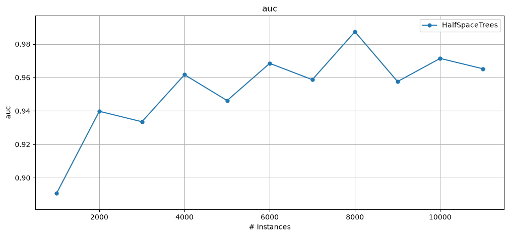
In this example, we use the prequential_evaluation_anomaly function with plot_windowed_results to plot AUC for HalfSpaceTrees on the synthetic data stream.

from capymoa.anomaly import HalfSpaceTrees
from capymoa.evaluation import prequential_evaluation_anomaly
from capymoa.evaluation.visualization import plot_windowed_results

stream_ad = NumpyStream(
    X,
    y,
    dataset_name="AnomalyDetectionDataset",
    feature_names=feature_names,
    target_name=target_name,
    target_type="categorical",
)
hst = HalfSpaceTrees(schema=stream_ad.get_schema())

results_hst = prequential_evaluation_anomaly(
    stream=stream_ad, learner=hst, window_size=1000
)

print(f"AUC: {results_hst.auc()}")
display(results_hst.windowed.metrics_per_window())
plot_windowed_results(results_hst, metric="auc", save_only=False)

AUC: 0.945191

	instances	auc	s_auc	Accuracy	Kappa	Periodical holdout AUC	Pos/Neg ratio	G-Mean	Recall	KappaM
0	1000.0	0.890795	0.190935	0.061	0.000996	0.000000	0.009082	0.229068	1.0	-103.333333
1	2000.0	0.939792	0.203641	0.011	0.000000	0.890795	0.011122	0.000000	1.0	-97.900000
2	3000.0	0.933535	0.176022	0.007	0.000000	0.939792	0.007049	0.000000	1.0	-109.333333
3	4000.0	0.961655	0.206375	0.009	0.000000	0.933535	0.009082	0.000000	1.0	-109.111111
4	5000.0	0.946188	0.195086	0.012	0.000000	0.961655	0.012146	0.000000	1.0	-101.916667
5	6000.0	0.968455	0.221530	0.012	0.000000	0.946188	0.012146	0.000000	1.0	-97.800000
6	7000.0	0.958694	0.212563	0.013	0.000000	0.968455	0.013171	0.000000	1.0	-93.643836
7	8000.0	0.987374	0.195112	0.010	0.000000	0.958694	0.010101	0.000000	1.0	-94.421687
8	9000.0	0.957560	0.200997	0.007	0.000000	0.987374	0.007049	0.000000	1.0	-98.300000
9	10000.0	0.971409	0.193359	0.009	0.000000	0.957560	0.009082	0.000000	1.0	-99.101010
10	10100.0	0.965222	0.199206	0.008	0.000000	0.971409	0.008065	0.000000	1.0	-99.192000

Autoencoder

from capymoa.anomaly import Autoencoder
from capymoa.evaluation import prequential_evaluation_anomaly
from capymoa.evaluation.visualization import plot_windowed_results

stream_ad = NumpyStream(
    X,
    y,
    dataset_name="AnomalyDetectionDataset",
    feature_names=feature_names,
    target_name=target_name,
    target_type="categorical",
)
ae = Autoencoder(schema=stream_ad.get_schema(), hidden_layer=1)

results_ae = prequential_evaluation_anomaly(
    stream=stream_ad, learner=ae, window_size=1000
)

print(f"AUC: {results_ae.auc()}")
display(results_ae.windowed.metrics_per_window())
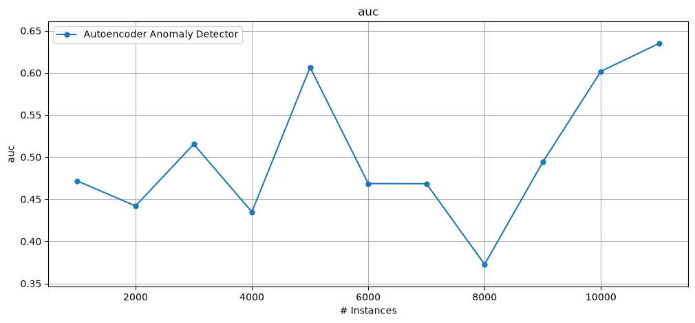
plot_windowed_results(results_ae, metric="auc", save_only=False)

AUC: 0.490696

	instances	auc	s_auc	Accuracy	Kappa	Periodical holdout AUC	Pos/Neg ratio	G-Mean	Recall	KappaM
0	1000.0	0.471690	-0.120168	0.009	0.000000	0.000000	0.009082	0.000000	1.000000	-109.111111
1	2000.0	0.442044	-0.098741	0.013	0.000045	0.471690	0.011122	0.044969	1.000000	-97.700000
2	3000.0	0.515322	-0.109961	0.007	0.000000	0.442044	0.007049	0.000000	1.000000	-109.333333
3	4000.0	0.434970	-0.093011	0.009	0.000000	0.515322	0.009082	0.000000	1.000000	-109.111111
4	5000.0	0.606444	-0.216212	0.012	0.000000	0.434970	0.012146	0.000000	1.000000	-101.916667
5	6000.0	0.468581	-0.120821	0.012	0.000000	0.606444	0.012146	0.000000	1.000000	-97.800000
6	7000.0	0.468475	-0.125352	0.012	-0.002002	0.468581	0.013171	0.000000	0.923077	-93.739726
7	8000.0	0.372727	-0.076485	0.010	-0.001984	0.468475	0.010101	0.030151	0.900000	-94.421687
8	9000.0	0.494102	-0.111006	0.009	0.000028	0.372727	0.007049	0.044879	1.000000	-98.100000
9	10000.0	0.601805	-0.181133	0.009	0.000000	0.494102	0.009082	0.000000	1.000000	-99.101010
10	10100.0	0.634892	-0.205302	0.008	0.000000	0.601805	0.008065	0.000000	1.000000	-99.192000

Online Isolation Forest

from capymoa.anomaly import OnlineIsolationForest
from capymoa.evaluation import prequential_evaluation_anomaly
from capymoa.evaluation.visualization import plot_windowed_results

stream_ad = NumpyStream(
    X,
    y,
    dataset_name="AnomalyDetectionDataset",
    feature_names=feature_names,
    target_name=target_name,
    target_type="categorical",
)
oif = OnlineIsolationForest(schema=stream_ad.get_schema(), num_trees=10)

results_oif = prequential_evaluation_anomaly(
    stream=stream_ad, learner=oif, window_size=1000
)

print(f"AUC: {results_oif.auc()}")
display(results_oif.windowed.metrics_per_window())
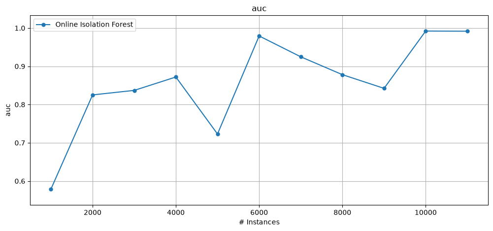
plot_windowed_results(results_oif, metric="auc", save_only=False)

AUC: 0.839909

	instances	auc	s_auc	Accuracy	Kappa	Periodical holdout AUC	Pos/Neg ratio	G-Mean	Recall	KappaM
0	1000.0	0.578989	0.027800	0.958	-0.014346	0.000000	0.009082	0.0	0.0	-3.666667
1	2000.0	0.825168	0.032921	0.989	0.000000	0.578989	0.011122	0.0	0.0	-0.100000
2	3000.0	0.837002	0.057356	0.993	0.000000	0.825168	0.007049	0.0	0.0	0.222222
3	4000.0	0.871959	0.041948	0.991	0.000000	0.837002	0.009082	0.0	0.0	0.000000
4	5000.0	0.723009	0.041858	0.988	0.000000	0.871959	0.012146	0.0	0.0	-0.250000
5	6000.0	0.979335	0.062274	0.988	0.000000	0.723009	0.012146	0.0	0.0	-0.200000
6	7000.0	0.924792	0.055090	0.987	0.000000	0.979335	0.013171	0.0	0.0	-0.246575
7	8000.0	0.878081	0.027914	0.990	0.000000	0.924792	0.010101	0.0	0.0	0.036145
8	9000.0	0.842325	0.045319	0.993	0.000000	0.878081	0.007049	0.0	0.0	0.300000
9	10000.0	0.992152	0.079348	0.991	0.000000	0.842325	0.009082	0.0	0.0	0.090909
10	10100.0	0.991683	0.083096	0.992	0.000000	0.992152	0.008065	0.0	0.0	0.192000

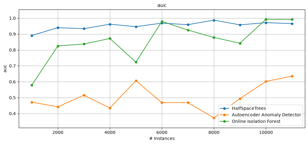
Comparing algorithms

plot_windowed_results(
    results_hst, results_ae, results_oif, metric="auc", save_only=False
)