Evaluating regressors in CapyMOA

This notebook further explores high-level evaluation functions as applied to regressors.

• High-level evaluation functions

  • We use prequential_evaluation() and prequential_evaluation_multiple_learners(), the same functions introduced for classification (see notebooks/classifier/evaluation.py), and show how they apply to regression with only minor differences.

  • We also show how to plot predictions vs. ground truth over time, which is particularly useful for regression tasks.

---

More information about CapyMOA can be found at https://www.capymoa.org.

last update on 28/11/2025

Regression

• We introduce a simple example using regression just to show how similar it is to assess regressors using the high-level evaluation functions.

• In the example below, we just use prequential_evaluation() but it would work with cumulative_evaluation() and windowed_evaluation() as well.

• One difference between classification and regression evaluation in CapyMOA is that the evaluators are different. Instead of ClassificationEvaluator and ClassificationWindowedEvaluator functions use RegressionEvaluator and RegressionWindowedEvaluator.

from capymoa.datasets import Fried
from capymoa.evaluation import prequential_evaluation
from capymoa.evaluation.visualization import plot_windowed_results
from capymoa.regressor import AdaptiveRandomForestRegressor, KNNRegressor

stream = Fried()
kNN_learner = KNNRegressor(schema=stream.get_schema(), k=5)
ARF_learner = AdaptiveRandomForestRegressor(
    schema=stream.get_schema(), ensemble_size=10
)

kNN_results = prequential_evaluation(
    stream=stream, learner=kNN_learner, window_size=5000
)
ARF_results = prequential_evaluation(
    stream=stream, learner=ARF_learner, window_size=5000
)

print(
    f"{kNN_results['learner']} [cumulative] RMSE = {kNN_results['cumulative'].rmse()} and \
    {ARF_results['learner']}  [cumulative] RMSE = {ARF_results['cumulative'].rmse()}"
)

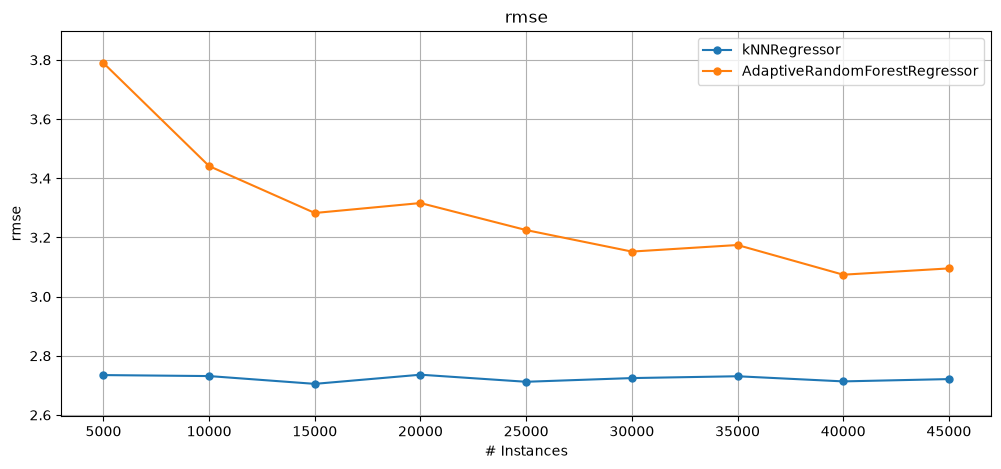
plot_windowed_results(kNN_results, ARF_results, metric="rmse")

kNNRegressor [cumulative] RMSE = 2.7229994765160916 and     AdaptiveRandomForestRegressor  [cumulative] RMSE = 3.312901313632365

Evaluating a single stream using multiple learners

• prequential_evaluation_multiple_learners also works for multiple regressors; the example below shows how it can be used.

from capymoa.evaluation import prequential_evaluation_multiple_learners

# Define the learners + an alias (dictionary key)
learners = {
    "kNNReg_k5": KNNRegressor(schema=stream.get_schema(), k=5),
    "kNNReg_k2": KNNRegressor(schema=stream.get_schema(), k=2),
    "kNNReg_k5_median": KNNRegressor(schema=stream.get_schema(), CLI="-k 5 -m"),
    "ARFReg_s5": AdaptiveRandomForestRegressor(
        schema=stream.get_schema(), ensemble_size=5
    ),
}

results = prequential_evaluation_multiple_learners(stream, learners)

print("Cumulative results for each learner:")
for learner_id in learners:
    if learner_id in results:
        cumulative = results[learner_id]["cumulative"]
        print(
            f"{learner_id}, RMSE: {cumulative.rmse():.2f}, adjusted R2: {cumulative.adjusted_r2():.2f}"
        )

# Tip: invoking metrics_header() from an evaluator will show us all the metrics available,
# e.g. results['kNNReg_k5']['cumulative'].metrics_header()
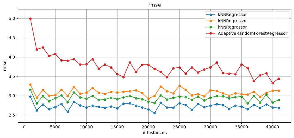
plot_windowed_results(
    results["kNNReg_k5"],
    results["kNNReg_k2"],
    results["kNNReg_k5_median"],
    results["ARFReg_s5"],
    metric="rmse",
)

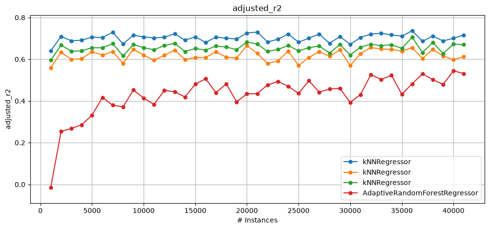
plot_windowed_results(
    results["kNNReg_k5"],
    results["kNNReg_k2"],
    results["kNNReg_k5_median"],
    results["ARFReg_s5"],
    metric="adjusted_r2",
)

Cumulative results for each learner:
kNNReg_k5, RMSE: 2.72, adjusted R2: 0.70
kNNReg_k2, RMSE: 3.08, adjusted R2: 0.62
kNNReg_k5_median, RMSE: 2.94, adjusted R2: 0.65
ARFReg_s5, RMSE: 3.77, adjusted R2: 0.43

Plotting predictions vs. ground truth over time

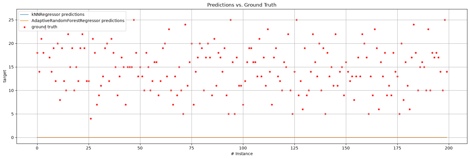
• In regression it is sometimes desirable to plot predictions vs. ground truth to observe what is happening with the stream. If we create a custom loop and use the evaluators directly, it is trivial to store the ground truth and predictions, and then proceed to plot them. However, to make people’s life easier the plot_predictions_vs_ground_truth function can be used.

• For massive streams with millions of instances, it can be unbearable to plot all at once, thus we can specify a plot_interval (that we want to investigate) to plot_predictions_vs_ground_truth. By default, the plot function will attempt to plot everything, i.e. with plot_interval=None, which is seldom a good idea.

from capymoa.datasets import Fried
from capymoa.evaluation import prequential_evaluation
from capymoa.evaluation.visualization import plot_predictions_vs_ground_truth
from capymoa.regressor import AdaptiveRandomForestRegressor, KNNRegressor

stream = Fried()
kNN_learner = KNNRegressor(schema=stream.get_schema(), k=5)
ARF_learner = AdaptiveRandomForestRegressor(
    schema=stream.get_schema(), ensemble_size=10
)

# When we specify store_predictions and store_y, the results will also include all the predictions and all the ground truth y.
# It is useful for debugging and outputting the predictions elsewhere.
kNN_results = prequential_evaluation(
    stream=stream,
    learner=kNN_learner,
    window_size=5000,
    store_predictions=True,
    store_y=True,
)
# We don't need to store the ground-truth for every experiment, since it is always the same for the same stream.
ARF_results = prequential_evaluation(
    stream=stream, learner=ARF_learner, window_size=5000, store_predictions=True
)


# Plot only 200 predictions (see plot_interval).
plot_predictions_vs_ground_truth(
    kNN_results,
    ARF_results,
    ground_truth=kNN_results["ground_truth_y"],
    plot_interval=(0, 200),
)