Evaluating classifiers in CapyMOA

This notebook further explores high-level evaluation functions, data abstraction and classifiers.

• High-level evaluation functions

  • We demonstrate how to use prequential_evaluation() and how to further encapsulate prequential evaluation using prequential_evaluation_multiple_learners.

  • We also discuss particularities about how these evaluation functions relate to how research has developed in the field, and how evaluation is commonly performed and presented.

• Supervised Learning

  • We clarify important information concerning the usage of classifiers and their predictions.

  • For the equivalent walkthrough using regressors, see notebooks/regressor/evaluation.py.

---

More information about CapyMOA can be found at https://www.capymoa.org.

last update on 28/11/2025

The difference between evaluators

• The following example implements a while loop that updates a ClassificationWindowedEvaluator and a ClassificationEvaluator for the same learner.

• The ClassificationWindowedEvaluator updates the metrics according to tumbling windows which ‘forgets’ older correct and incorrect predictions. This allows us to observe how well the learner performs in shorter windows.

• The ClassificationEvaluator updates the metrics, taking into account all the correct and incorrect predictions made. It is useful to observe the overall performance after processing hundreds of thousands of instances.

• Two important points:

  1. Regarding window_size in ClassificationEvaluator: A ClassificationEvaluator also allows us to specify a window size, but it only controls the frequency at which cumulative metrics are calculated.

  2. If we access metrics directly (not through metrics_per_window()) in ClassificationWindowedEvaluator we will be looking at the metrics corresponding to the last window.

For further insight into the specifics of the evaluators, please refer to the documentation at https://www.capymoa.org.

from capymoa.classifier import AdaptiveRandomForestClassifier
from capymoa.datasets import Electricity
from capymoa.evaluation import ClassificationEvaluator, ClassificationWindowedEvaluator

stream = Electricity()

ARF = AdaptiveRandomForestClassifier(schema=stream.get_schema(), ensemble_size=10)

# The window_size in ClassificationWindowedEvaluator specifies the amount of instances used per evaluation.
windowedEvaluatorARF = ClassificationWindowedEvaluator(
    schema=stream.get_schema(), window_size=4500
)
# The window_size ClassificationEvaluator just specifies the frequency at which the cumulative metrics are stored.
classificationEvaluatorARF = ClassificationEvaluator(
    schema=stream.get_schema(), window_size=4500
)

while stream.has_more_instances():
    instance = stream.next_instance()
    prediction = ARF.predict(instance)
    windowedEvaluatorARF.update(instance.y_index, prediction)
    classificationEvaluatorARF.update(instance.y_index, prediction)
    ARF.train(instance)

# Showing only the 'classifications correct (percent)' (i.e. accuracy)
print(
    "[ClassificationWindowedEvaluator] Windowed accuracy reported for every window_size windows"
)
print(windowedEvaluatorARF.accuracy())

print(
    f"[ClassificationEvaluator] Cumulative accuracy: {classificationEvaluatorARF.accuracy()}"
)
# We could report the cumulative accuracy every window_size instances with the following code, but that is normally not very insightful.
# display(classificationEvaluatorARF.metrics_per_window())

[ClassificationWindowedEvaluator] Windowed accuracy reported for every window_size windows
[89.57777777777778, 89.46666666666667, 90.2, 89.71111111111111, 88.68888888888888, 88.48888888888888, 87.6888888888889, 88.88888888888889, 89.28888888888889, 91.06666666666666]
[ClassificationEvaluator] Cumulative accuracy: 89.32953742937853

High-level evaluation functions

In CapyMOA, for supervised learning, there is one primary evaluation function designed to handle the manipulation of evaluators, i.e. the prequential_evaluation(). This function streamlines the process, ensuring users need not directly update them. Essentially, this function executes the evaluation loop and updates the relevant evaluators:

• prequential_evaluation() utilises ClassificationEvaluator and ClassificationWindowedEvaluator.

Previously, CapyMOA included two other functions: cumulative_evaluation() and windowed_evaluation(). However, since prequential_evaluation() incorporates the functionality of both we decided to remove those functions and focus on prequential_evaluation(). It’s important to note that prequential_evaluation() is applicable to both Regression and Prediction Intervals besides Classification. The functionality and interpretation remain the same across these cases, but the metrics differ.

Result of a high-level function

• The return from prequential_evaluation() is a PrequentialResults object which provides access to the cumulative and windowed metrics as well as some other metrics (like wall-clock and cpu time).

Common characteristics for all high-level evaluation functions

• prequential_evaluation() specifies a max_instances parameter, which by default is None. Depending on the source of the data (e.g. a real stream or a synthetic stream) the function will never stop! The intuition behind this is that streams are infinite, we process them as such. Therefore, it is a good idea to specify max_instances unless you are using a snapshot of a stream (i.e. a Dataset like Electricity)

Evaluation practices in the literature (and practice)

Interested readers might want to peruse section 6.1.1 Error Estimation from Machine Learning for Data Streams book. We further expand the relationships between the literature and our evaluation functions in the documentation: https://www.capymoa.org.

prequential_evaluation()

The prequential_evaluation() function performs a windowed evaluation and a cumulative evaluation at once. Internally, it maintains a ClassificationWindowedEvaluator (for the windowed metrics) and ClassificationEvaluator (for the cumulative metrics). This allows us to have access to the cumulative and windowed results without running two separate evaluation functions.

• The results returned from prequential_evaluation() allows access to the evaluator objects ClassificationWindowedEvaluator (attribute windowed) and ClassificationEvaluator (attribute cumulative) directly.

• Notice that the computational overhead of training and assessing the same model twice outweighs the minimum overhead of updating the two evaluators within the function. Thus, it is advisable to use the prequential_evaluation() function instead of creating separate while loops for evaluation.

• Advanced users might intuitively request metrics directly from the results object, which will return the cumulative metrics. For example, assuming results = prequential_evaluation(...), results.accuracy() will return the cumulative accuracy. IMPORTANT: There are no IDE hints for these metrics as they are accessed dynamically via __getattr__. It is advisable that users access metrics explicitly through results.cumulative (or results['cumulative']) or results.windowed (or results['windowed']).

• Invoking results.metrics_per_window() from a results object will return the dataframe with the windowed results.

• results.write_to_file() will output the cumulative and windowed results to a directory.

• results.cumulative.metrics_dict() will return all the cumulative metrics identifiers and their corresponding values in a dictionary structure.

• Invoking plot_windowed_results() with a PrequentialResults object will plot its windowed results.

• For plotting and analysis purposes, one might want to set store_predictions=True and store_y=True on the prequential_evaluation() function, which will include all the predictions and ground truth y in the PrequentialResults object. It is important to note that this can be costly in terms of memory depending on the size of the stream.

from capymoa.classifier import HoeffdingTree
from capymoa.datasets import ElectricityTiny
from capymoa.evaluation import prequential_evaluation
from capymoa.evaluation.visualization import plot_windowed_results

elec_stream = ElectricityTiny()
ht = HoeffdingTree(schema=elec_stream.get_schema(), grace_period=50)

results_ht = prequential_evaluation(
    stream=elec_stream,
    learner=ht,
    window_size=100,
    optimise=True,
    store_predictions=False,
    store_y=False,
)


print("\tDifferent ways of accessing metrics:")

print(
    f"results_ht['wallclock']: {results_ht['wallclock']} results_ht.wallclock(): {results_ht.wallclock()}"
)
print(
    f"results_ht['cpu_time']: {results_ht['cpu_time']} results_ht.cpu_time(): {results_ht.cpu_time()}"
)

print(f"results_ht.cumulative.accuracy() = {results_ht.cumulative.accuracy()}")
print(f"results_ht.cumulative['accuracy'] = {results_ht.cumulative['accuracy']}")
print(f"results_ht['cumulative'].accuracy() = {results_ht['cumulative'].accuracy()}")
print(f"results_ht.accuracy() = {results_ht.accuracy()}")

print("\n\tAll the cumulative results:")
print(results_ht.cumulative.metrics_dict())

print("\n\tAll the windowed results:")
display(results_ht.metrics_per_window())
# OR display(results_ht.windowed.metrics_per_window())

# results_ht.write_to_file() -> this will save the results to a directory

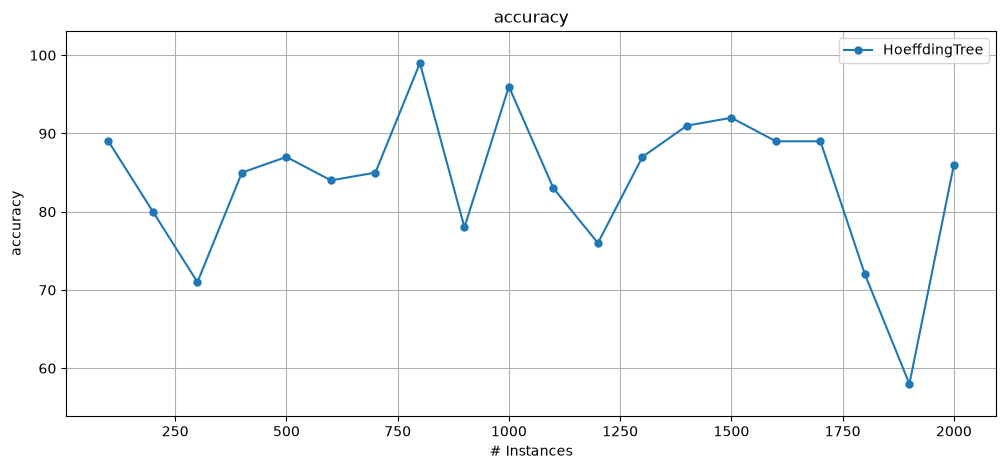
plot_windowed_results(results_ht, metric="accuracy")

	Different ways of accessing metrics:
results_ht['wallclock']: 0.030479907989501953 results_ht.wallclock(): 0.030479907989501953
results_ht['cpu_time']: 0.1046382219999984 results_ht.cpu_time(): 0.1046382219999984
results_ht.cumulative.accuracy() = 83.85000000000001
results_ht.cumulative['accuracy'] = 83.85000000000001
results_ht['cumulative'].accuracy() = 83.85000000000001
results_ht.accuracy() = 83.85000000000001

	All the cumulative results:
{'instances': 2000.0, 'accuracy': 83.85000000000001, 'kappa': 66.04003700899992, 'kappa_t': -14.946619217081869, 'kappa_m': 59.010152284263974, 'f1_score': 83.85000000000001, 'F1 Score macro (percent)': 83.01676424140277, 'f1_score_0': 86.77855096193205, 'f1_score_1': 79.25497752087348, 'precision': 83.85000000000001, 'Precision macro (percent)': 83.24177714270593, 'precision_0': 85.82995951417004, 'precision_1': 80.65359477124183, 'recall': 83.85000000000001, 'Recall macro (percent)': 82.82619238745067, 'recall_0': 87.74834437086093, 'recall_1': 77.90404040404042, 'roc_auc': 0.9265178690882333}

	All the windowed results:

	instances	accuracy	kappa	kappa_t	kappa_m	f1_score	F1 Score macro (percent)	f1_score_0	f1_score_1	precision	Precision macro (percent)	precision_0	precision_1	recall	Recall macro (percent)	recall_0	recall_1	roc_auc
0	100.0	89.0	75.663717	31.250000	64.516129	89.0	87.830512	91.603053	84.057971	89.0	87.582418	92.307692	82.857143	89.0	88.101604	90.909091	85.294118	0.963458
1	200.0	80.0	49.367089	-42.857143	67.213115	80.0	73.333333	60.000000	86.666667	80.0	88.235294	100.000000	76.470588	80.0	71.428571	42.857143	100.000000	0.966247
2	300.0	71.0	16.953036	-141.666667	29.268293	71.0	58.422939	81.290323	35.555556	71.0	58.114035	82.894737	33.333333	71.0	58.921037	79.746835	38.095238	0.926065
3	400.0	85.0	66.637011	-36.363636	77.941176	85.0	83.166872	77.611940	88.721805	85.0	86.376882	89.655172	83.098592	85.0	81.791171	68.421053	95.161290	0.930663
4	500.0	87.0	73.684211	-8.333333	80.000000	87.0	86.776523	88.495575	85.057471	87.0	87.916667	83.333333	92.500000	87.0	86.531513	94.339623	78.723404	0.925619
5	600.0	84.0	64.221825	-14.285714	54.285714	84.0	81.908639	88.059701	75.757576	84.0	85.615079	81.944444	89.285714	84.0	80.475382	95.161290	65.789474	0.918610
6	700.0	85.0	70.000000	16.666667	70.588235	85.0	84.816277	83.146067	86.486486	85.0	85.000000	74.000000	96.000000	85.0	86.780160	94.871795	78.688525	0.913823
7	800.0	99.0	97.954173	94.117647	97.674419	99.0	98.976982	98.823529	99.130435	99.0	99.137931	100.000000	98.275862	99.0	98.837209	97.674419	100.000000	0.927805
8	900.0	78.0	57.446809	-15.789474	56.862745	78.0	77.678571	80.357143	75.000000	78.0	83.582090	67.164179	100.000000	78.0	80.000000	100.000000	60.000000	0.926853
9	1000.0	96.0	91.922456	50.000000	92.727273	96.0	95.959596	95.555556	96.363636	96.0	96.185065	97.727273	94.642857	96.0	95.813205	93.478261	98.148148	0.933932
10	1100.0	83.0	1.162791	-142.857143	0.000000	83.0	50.567025	90.607735	10.526316	83.0	50.555556	91.111111	10.000000	83.0	50.610501	90.109890	11.111111	0.933736
11	1200.0	76.0	10.979228	-100.000000	7.692308	76.0	50.166113	86.046512	14.285714	76.0	87.755102	75.510204	100.000000	76.0	53.846154	100.000000	7.692308	0.932933
12	1300.0	87.0	66.529351	-62.500000	59.375000	87.0	82.892486	91.275168	74.509804	87.0	91.975309	83.950617	100.000000	87.0	79.687500	100.000000	59.375000	0.935017
13	1400.0	91.0	64.285714	57.142857	52.631579	91.0	81.851180	94.736842	68.965517	91.0	95.000000	90.000000	100.000000	91.0	76.315789	100.000000	52.631579	0.939230
14	1500.0	92.0	62.686567	42.857143	50.000000	92.0	81.060606	95.454545	66.666667	92.0	95.652174	91.304348	100.000000	92.0	75.000000	100.000000	50.000000	0.942960
15	1600.0	89.0	73.170732	21.428571	65.625000	89.0	86.504723	92.307692	80.701754	89.0	90.000000	88.000000	92.000000	89.0	84.466912	97.058824	71.875000	0.944120
16	1700.0	89.0	78.000000	8.333333	76.086957	89.0	88.972431	89.523810	88.421053	89.0	89.393939	85.454545	93.333333	89.0	89.000000	94.000000	84.000000	0.944423
17	1800.0	72.0	45.141066	-47.368421	9.677419	72.0	70.288625	63.157895	77.419355	72.0	81.578947	100.000000	63.157895	72.0	73.076923	46.153846	100.000000	0.936524
18	1900.0	58.0	24.677188	-200.000000	-31.250000	58.0	57.983193	58.823529	57.142857	58.0	65.329768	88.235294	42.424242	58.0	65.808824	44.117647	87.500000	0.927778
19	2000.0	86.0	66.410749	26.315789	58.823529	86.0	83.001457	90.140845	75.862069	86.0	87.938596	84.210526	91.666667	86.0	80.837790	96.969697	64.705882	0.926518

Evaluating a single stream using multiple learners

prequential_evaluation_multiple_learners() further encapsulates experiments by executing multiple learners on a single stream.

• This function behaves as if we invoked prequential_evaluation() multiple times, but internally it only iterates through the stream once. This is useful if we are faced with a situation where accessing each instance of the stream is costly, then this function will be more convenient than just invoking prequential_evaluation() multiple times.

• This method does not calculate wallclock or cpu_time because the training and testing of each learner is interleaved, thus timing estimations are unreliable. Thus, the results dictionaries do not contain the keys wallclock and cpu_time.

from capymoa.classifier import AdaptiveRandomForestClassifier, OnlineBagging
from capymoa.datasets import Electricity
from capymoa.evaluation import prequential_evaluation_multiple_learners
from capymoa.evaluation.visualization import plot_windowed_results

stream = Electricity()

# Define the learners + an alias (dictionary key)
learners = {
    "OB": OnlineBagging(schema=stream.get_schema(), ensemble_size=10),
    "ARF": AdaptiveRandomForestClassifier(schema=stream.get_schema(), ensemble_size=10),
}

results = prequential_evaluation_multiple_learners(stream, learners, window_size=4500)

print(
    f"OB final accuracy = {results['OB'].cumulative.accuracy()} and ARF final accuracy = {results['ARF'].cumulative.accuracy()}"
)
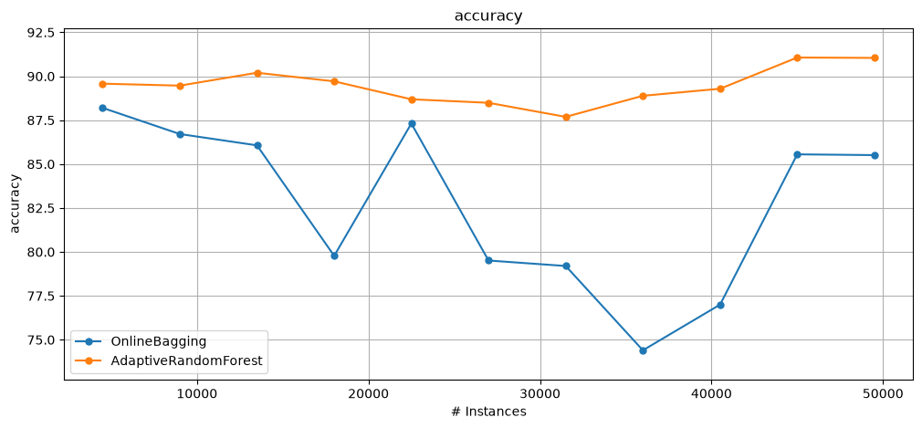
plot_windowed_results(results["OB"], results["ARF"], metric="accuracy")

OB final accuracy = 82.4174611581921 and ARF final accuracy = 89.32953742937853