Getting started with classification#
This notebook shows some basic usage of CapyMOA for streaming classification.
There are more detailed notebooks and documentation available; our goal here is just to present some high-level functions and demonstrate a subset of CapyMOA’s functionalities.
For simplicity, we simulate data streams in the following examples using datasets and employing synthetic generators. One could also read data directly from a CSV or ARFF (See stream_from_file function).
More information about CapyMOA can be found at https://www.capymoa.org
last update on 05/08/2026
Test-then-train loop#
Classification for data streams traditionally assumes instances are available to the classifier in an incremental fashion and labels become available before a new instance becomes available.
It is common to simulate this behavior using a while loop, often referred to as a test-then-train loop which contains 4 distinct steps:
Fetches the next instance from the stream
Makes a prediction
Train the model with the instance
Update a mechanism to keep track of metrics
Some remarks about the test-then-train loop:
We must not train before testing, meaning that steps 2 and 3 should not be interchanged, as this would invalidate our interpretation concerning how the model performs on unseen data, leading to unreliable evaluations of its efficacy.
Steps 3 and 4 can be completed in any order without altering the result.
What if labels are not immediately available? Then you might want to read about delayed labeling and partially labeled data, see A Survey on Semi-supervised Learning for Delayed Partially Labelled Data Streams
More information on classification for data streams is available at section 2.2 Classification from the Machine Learning for Data Streams book
from capymoa.classifier import OnlineBagging
from capymoa.datasets import Electricity
from capymoa.evaluation import ClassificationEvaluator

elec_stream = Electricity()
ob_learner = OnlineBagging(schema=elec_stream.get_schema(), ensemble_size=5)
ob_evaluator = ClassificationEvaluator(schema=elec_stream.get_schema())

for instance in elec_stream:
    prediction = ob_learner.predict(instance)
    ob_learner.train(instance)
    ob_evaluator.update(instance.y_index, prediction)

print(ob_evaluator.accuracy())
82.06656073446328
High-level evaluation functions#
If our goal is just to evaluate learners, it would be tedious to keep writing test-then-train loops. Thus, it makes sense to encapsulate that loop inside high-level evaluation functions.
Furthermore, sometimes we are interested in cumulative metrics and sometimes we care about windowed metrics. For example, if we want to know how accurate our model is so far, considering all the instances it has seen, then we would look at its cumulative metrics. However, we might also be interested in how well the model is performing every n number of instances, so that we can, for example, identify periods in which our model was really struggling to produce correct predictions.
In this example, we use the
prequential_evaluationfunction, which provides us with both the cumulative and the windowed metrics!Some remarks:
If you want to know more about other high-level evaluation functions, evaluators, or which metrics are available, check the evaluation notebook (notebooks/classifier/evaluation.py).
The results from evaluation functions such as prequential_evaluation follow a standard and are discussed thoroughly in the Evaluation documentation at http://www.capymoa.org.
Sometimes authors refer to the cumulative metrics as test-then-train metrics, such as test-then-train accuracy (or TTT accuracy for short). They all refer to the same concept.
Shouldn’t we recreate the stream object
elec_stream? No,prequential_evaluation(), by default, will automaticallyrestart()streams when they are reused.
In the below example prequential_evaluation is used with a HoeffdingTree classifier on the Electricity data stream.
from capymoa.classifier import HoeffdingTree
from capymoa.evaluation import prequential_evaluation

ht = HoeffdingTree(schema=elec_stream.get_schema(), grace_period=50)

# Obtain the results from the high-level function.
# Note that we need to specify a window_size as we obtain both windowed and cumulative results.
# The results from a high-level evaluation function are represented as a PrequentialResults object.
results_ht = prequential_evaluation(stream=elec_stream, learner=ht, window_size=4500)

print(
    f"Cumulative accuracy = {results_ht.cumulative.accuracy()}, wall-clock time: {results_ht.wallclock()}"
)

# The windowed results are conveniently stored in a pandas DataFrame.
display(results_ht.windowed.metrics_per_window())
Cumulative accuracy = 81.6604872881356, wall-clock time: 0.33509325981140137
| instances | accuracy | kappa | kappa_t | kappa_m | f1_score | F1 Score macro (percent) | f1_score_0 | f1_score_1 | precision | Precision macro (percent) | precision_0 | precision_1 | recall | Recall macro (percent) | recall_0 | recall_1 | roc_auc | |
|---|---|---|---|---|---|---|---|---|---|---|---|---|---|---|---|---|---|---|
| 0 | 4500.0 | 87.777778 | 74.440796 | 24.242424 | 68.856172 | 87.777778 | 87.220134 | 84.550562 | 89.889706 | 87.777778 | 87.149807 | 84.078212 | 90.221402 | 87.777778 | 87.294344 | 85.028249 | 89.560440 | 0.937830 |
| 1 | 9000.0 | 83.666667 | 66.963969 | 2.649007 | 64.458414 | 83.666667 | 83.468246 | 81.657100 | 85.279391 | 83.666667 | 83.752489 | 84.373388 | 83.131589 | 83.666667 | 83.325685 | 79.110251 | 87.541118 | 0.917425 |
| 2 | 13500.0 | 85.644444 | 71.282626 | 2.269289 | 70.009285 | 85.644444 | 85.636773 | 85.304823 | 85.968723 | 85.644444 | 85.634554 | 83.780161 | 87.488948 | 85.644444 | 85.693216 | 86.886006 | 84.500427 | 0.915233 |
| 3 | 18000.0 | 81.977778 | 61.953129 | -25.154321 | 57.021728 | 81.977778 | 80.839091 | 76.168087 | 85.510095 | 81.977778 | 82.841248 | 85.488127 | 80.194370 | 81.977778 | 80.130502 | 68.680445 | 91.580559 | 0.905326 |
| 4 | 22500.0 | 86.177778 | 70.202882 | 13.370474 | 64.719229 | 86.177778 | 85.045965 | 80.931944 | 89.159986 | 86.177778 | 86.648480 | 88.058706 | 85.238254 | 86.177778 | 84.166185 | 74.872377 | 93.459993 | 0.905125 |
| 5 | 27000.0 | 78.088889 | 53.951820 | -72.377622 | 47.272727 | 78.088889 | 76.892339 | 71.634062 | 82.150615 | 78.088889 | 77.962693 | 77.521793 | 78.403594 | 78.088889 | 76.425652 | 66.577540 | 86.273764 | 0.895114 |
| 6 | 31500.0 | 79.066667 | 55.619360 | -71.897810 | 46.263548 | 79.066667 | 77.802243 | 72.504378 | 83.100108 | 79.066667 | 78.081099 | 74.237896 | 81.924301 | 79.066667 | 77.580064 | 70.849971 | 84.310157 | 0.887665 |
| 7 | 36000.0 | 74.955556 | 49.002474 | -89.411765 | 37.354086 | 74.955556 | 74.420210 | 70.719667 | 78.120753 | 74.955556 | 74.256346 | 66.390244 | 82.122449 | 74.955556 | 75.072035 | 75.653141 | 74.490929 | 0.879380 |
| 8 | 40500.0 | 74.555556 | 50.130218 | -71.664168 | 41.312148 | 74.555556 | 74.552780 | 74.818562 | 74.286998 | 74.555556 | 76.196815 | 65.523883 | 86.869748 | 74.555556 | 76.037125 | 87.186058 | 64.888191 | 0.871657 |
| 9 | 45000.0 | 84.377778 | 68.535062 | -0.428571 | 68.390288 | 84.377778 | 84.267355 | 82.949309 | 85.585401 | 84.377778 | 84.249034 | 82.648623 | 85.849445 | 84.377778 | 84.287584 | 83.252191 | 85.322976 | 0.872949 |
| 10 | 45312.0 | 84.266667 | 68.237903 | -2.757620 | 67.876588 | 84.266667 | 84.118949 | 82.587309 | 85.650588 | 84.266667 | 84.121918 | 82.627953 | 85.615883 | 84.266667 | 84.116013 | 82.546706 | 85.685320 | 0.873272 |
Comparing results among classifiers#
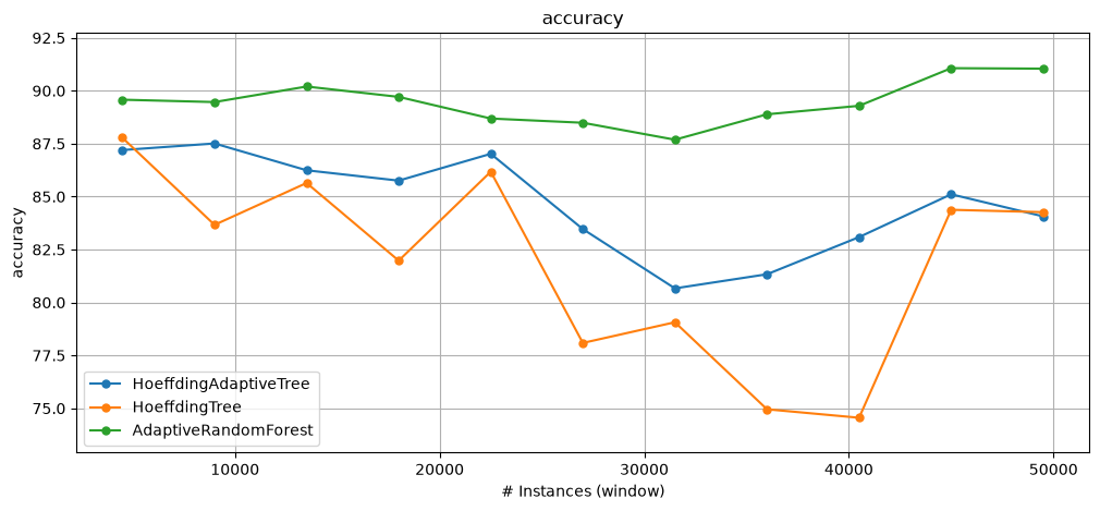
CapyMOA provides
plot_windowed_resultsas an easy visualisation function for quickly comparing windowed metrics.In the example below, we create three classifiers: HoeffdingAdaptiveTree, HoeffdingTree and AdaptiveRandomForest, and plot the results using
plot_windowed_results.More details about
plot_windowed_resultsoptions are described in the documentation at http://www.capymoa.org.
from moa.classifiers.trees import HoeffdingAdaptiveTree

from capymoa.base import MOAClassifier
from capymoa.classifier import AdaptiveRandomForestClassifier, HoeffdingTree
from capymoa.evaluation.visualization import plot_windowed_results

# Create the wrapper for HoeffdingAdaptiveTree (from MOA).
HAT = MOAClassifier(
    schema=elec_stream.get_schema(), moa_learner=HoeffdingAdaptiveTree, CLI="-g 50"
)
HT = HoeffdingTree(schema=elec_stream.get_schema(), grace_period=50)
ARF = AdaptiveRandomForestClassifier(
    schema=elec_stream.get_schema(), ensemble_size=10, number_of_jobs=4
)

results_HAT = prequential_evaluation(stream=elec_stream, learner=HAT, window_size=4500)
results_HT = prequential_evaluation(stream=elec_stream, learner=HT, window_size=4500)
results_ARF = prequential_evaluation(stream=elec_stream, learner=ARF, window_size=4500)

# Comparing models based on their cumulative accuracy.
print(f"HAT accuracy = {results_HAT.cumulative.accuracy()}")
print(f"HT accuracy = {results_HT.cumulative.accuracy()}")
print(f"ARF accuracy = {results_ARF.cumulative.accuracy()}")

# Plotting the results. Note that we ovewrote the ylabel, but that doesn't change the metric.
plot_windowed_results(
    results_HAT,
    results_HT,
    results_ARF,
    metric="accuracy",
    xlabel="# Instances (window)",
)
HAT accuracy = 84.68617584745762
HT accuracy = 81.6604872881356
ARF accuracy = 89.32953742937853
Concept drift#
One of the most challenging and defining aspects of data streams is the phenomenon known as concept drifts.
In CapyMOA, we designed the simplest and most complete API for simulating, visualising and assessing concept drifts.
In the example below, we focus on a simple way of simulating and visualising a drifting stream. There is a tutorial focusing entirely on how concept drift can be simulated, detected and assessed in a separate notebook (See notebooks/drift:
Simulating Concept Drifts with the DriftStream API).
Plotting drift detection results#
This example uses the DriftStream building API, precisely the positional version where drifts are specified according to their exact location in the stream.
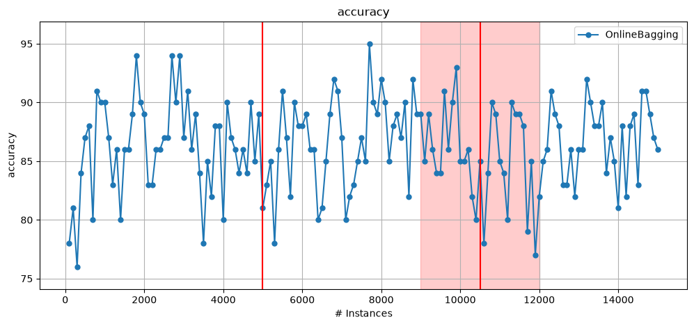
Integration with the visualisation function. The DriftStream object carries meta-information about the drift which is passed along the stream and thus becomes available to
plot_windowed_results.The following plot contains two drifts: 1 abrupt and 1 gradual, such that the abrupt drift is located at instance 5000 and the gradual drift starts at instance 9000 and ends at 12000. This information is provided to the stream via
GradualDrift(start=9000, end=12000).More details concerning concept drifts in CapyMOA can be found in the documentation at http://www.capymoa.org.
from capymoa.classifier import OnlineBagging
from capymoa.stream.drift import AbruptDrift, DriftStream, GradualDrift
from capymoa.stream.generator import SEA

# Generating a synthetic stream with 1 abrupt drift and 1 gradual drift.
stream_sea2drift = DriftStream(
    stream=[
        SEA(function=1),
        AbruptDrift(position=5000),
        SEA(function=3),
        GradualDrift(start=9000, end=12000),
        SEA(function=1),
    ]
)

OB = OnlineBagging(schema=stream_sea2drift.get_schema(), ensemble_size=10)

# Since this is a synthetic stream, max_instances is needed to determine the amount of instances to be generated.
results_sea2drift_OB = prequential_evaluation(
    stream=stream_sea2drift, learner=OB, window_size=100, max_instances=15000
)

plot_windowed_results(results_sea2drift_OB, metric="accuracy")