
Data Drift Detection in CapyMOA#
This tutorial shows how to detect data drift (changes in the input data
distribution) using detectors in capymoa.drift.detectors.
Unlike concept drift detectors, which track prediction errors, data drift detectors compare recent observations against a reference distribution to determine whether the data-generating process has changed.
In this tutorial we cover:
A first example with the Kolmogorov–Smirnov test.
Inspecting the
DataDriftResultobject.Comparing statistical test detectors (KS, Anderson–Darling, Cramér–von Mises).
Comparing distance-based detectors (KL, JS, PSI, Hellinger, Wasserstein, Energy Distance).
Multivariate detectors (MMD, D3, BNDM).
Categorical features with the Chi-Square test.
Batch comparison with
compare().Auto-fit mode for fully streaming workflows.
More information about CapyMOA can be found at https://www.capymoa.org.
last update on 15/09/2026
# This cell is hidden on capymoa.org. See docs/contributing/docs.rst
from capymoa._nbmock import is_nb_fast

# Reduce sizes when running in fast mode (CI / nbmake)
if is_nb_fast():
    _N_REF = 50
    _WINDOW = 20
    _STREAM_LEN = 100
else:
    _N_REF = 500
    _WINDOW = 100
    _STREAM_LEN = 800
import matplotlib.pyplot as plt
import numpy as np
import pandas as pd

rng = np.random.default_rng(42)
Synthetic data with a known drift#
We create a simple two-feature stream where the first half is drawn from
N(0, 1) and the second half shifts to N(3, 1). This makes it easy to
verify whether detectors fire at the right moment.
N_REF = _N_REF
WINDOW = _WINDOW
STREAM_LEN = _STREAM_LEN
N_FEATURES = 2
SHIFT = 3.0

# Reference data (stable distribution)
X_ref = rng.normal(0, 1, size=(N_REF, N_FEATURES))

# Streaming data: first half is same distribution, second half is shifted
half = STREAM_LEN // 2
X_stream = np.vstack(
    [
        rng.normal(0, 1, size=(half, N_FEATURES)),
        rng.normal(SHIFT, 1, size=(half, N_FEATURES)),
    ]
)

print(f"Reference: {X_ref.shape},  Stream: {X_stream.shape}")
print(f"Drift occurs at observation {half}")
Reference: (500, 2),  Stream: (800, 2)
Drift occurs at observation 400
1. A first example with Kolmogorov–Smirnov#
The Kolmogorov–Smirnov (KS) test compares the empirical CDFs of the reference and test windows, feature by feature. It is one of the simplest and most widely used univariate data-drift detectors.
The workflow is:
Fit the detector on a reference dataset.
Stream new observations one at a time with
add_element().Check for drift with
detected_change().
from capymoa.drift.detectors import KolmogorovSmirnov

ks = KolmogorovSmirnov(window_size=WINDOW)
ks.fit(X_ref)

detections = []
for i, x in enumerate(X_stream):
    ks.add_element(x)
    if ks.detected_change():
        detections.append(i)

print(f"KS detected drift at observations: {detections}")
print(f"(True drift is at observation {half})")
KS detected drift at observations: [408, 409, 410, 411, 412, 413, 414, 415, 416, 417, 418, 419, 420, 421, 422, 423, 424, 425, 426, 427, 428, 429, 430, 431, 432, 433, 434, 435, 436, 437, 438, 439, 440, 441, 442, 443, 444, 445, 446, 447, 448, 449, 450, 451, 452, 453, 454, 455, 456, 457, 458, 459, 460, 461, 462, 463, 464, 465, 466, 467, 468, 469, 470, 471, 472, 473, 474, 475, 476, 477, 478, 479, 480, 481, 482, 483, 484, 485, 486, 487, 488, 489, 490, 491, 492, 493, 494, 495, 496, 497, 498, 499, 500, 501, 502, 503, 504, 505, 506, 507, 508, 509, 510, 511, 512, 513, 514, 515, 516, 517, 518, 519, 520, 521, 522, 523, 524, 525, 526, 527, 528, 529, 530, 531, 532, 533, 534, 535, 536, 537, 538, 539, 540, 541, 542, 543, 544, 545, 546, 547, 548, 549, 550, 551, 552, 553, 554, 555, 556, 557, 558, 559, 560, 561, 562, 563, 564, 565, 566, 567, 568, 569, 570, 571, 572, 573, 574, 575, 576, 577, 578, 579, 580, 581, 582, 583, 584, 585, 586, 587, 588, 589, 590, 591, 592, 593, 594, 595, 596, 597, 598, 599, 600, 601, 602, 603, 604, 605, 606, 607, 608, 609, 610, 611, 612, 613, 614, 615, 616, 617, 618, 619, 620, 621, 622, 623, 624, 625, 626, 627, 628, 629, 630, 631, 632, 633, 634, 635, 636, 637, 638, 639, 640, 641, 642, 643, 644, 645, 646, 647, 648, 649, 650, 651, 652, 653, 654, 655, 656, 657, 658, 659, 660, 661, 662, 663, 664, 665, 666, 667, 668, 669, 670, 671, 672, 673, 674, 675, 676, 677, 678, 679, 680, 681, 682, 683, 684, 685, 686, 687, 688, 689, 690, 691, 692, 693, 694, 695, 696, 697, 698, 699, 700, 701, 702, 703, 704, 705, 706, 707, 708, 709, 710, 711, 712, 713, 714, 715, 716, 717, 718, 719, 720, 721, 722, 723, 724, 725, 726, 727, 728, 729, 730, 731, 732, 733, 734, 735, 736, 737, 738, 739, 740, 741, 742, 743, 744, 745, 746, 747, 748, 749, 750, 751, 752, 753, 754, 755, 756, 757, 758, 759, 760, 761, 762, 763, 764, 765, 766, 767, 768, 769, 770, 771, 772, 773, 774, 775, 776, 777, 778, 779, 780, 781, 782, 783, 784, 785, 786, 787, 788, 789, 790, 791, 792, 793, 794, 795, 796, 797, 798, 799]
(True drift is at observation 400)
2. Inspecting a DataDriftResult#
Instead of a simple boolean, you can call compare() on any test window
to get a full DataDriftResult. This object contains:
is_drift– overall drift decision.statistic– aggregated test statistic.p_value– aggregated p-value (for statistical tests).feature_is_drift– per-feature drift decisions.feature_statistics– per-feature test statistics.feature_p_values– per-feature p-values.
ks_fresh = KolmogorovSmirnov(window_size=WINDOW)
ks_fresh.fit(X_ref)

# Compare against the shifted portion of the stream
result = ks_fresh.compare(X_stream[half : half + WINDOW])

print(f"is_drift      : {result.is_drift}")
print(f"statistic     : {result.statistic:.4f}")
print(f"p_value       : {result.p_value:.2e}")
print(f"feature_drift : {result.feature_is_drift}")
print(f"feature_stats : {result.feature_statistics}")
print(f"feature_pvals : {result.feature_p_values}")
is_drift      : True
statistic     : 0.8560
p_value       : 8.68e-66
feature_drift : {0: np.True_, 1: np.True_}
feature_stats : {0: np.float64(0.856), 1: np.float64(0.846)}
feature_pvals : {0: np.float64(8.679952003291608e-66), 1: np.float64(9.21403121023077e-64)}
3. Statistical test detectors#
CapyMOA includes three univariate statistical-test detectors that produce p-values and use Bonferroni correction across features:
Detector |
Key idea |
|---|---|
KolmogorovSmirnov |
Max difference between empirical CDFs |
AndersonDarling |
Weighted CDF comparison (more sensitive in tails) |
CramerVonMises |
Integrated squared CDF difference |
We compare them on the same synthetic stream.
from capymoa.drift.detectors import (
    AndersonDarling,
    CramerVonMises,
    KolmogorovSmirnov,
)

stat_detectors = {
    "KS": KolmogorovSmirnov(window_size=WINDOW),
    "Anderson-Darling": AndersonDarling(window_size=WINDOW),
    "Cramér-von Mises": CramerVonMises(window_size=WINDOW),
}

results = {}
for name, det in stat_detectors.items():
    det.fit(X_ref)
    dets = []
    for i, x in enumerate(X_stream):
        det.add_element(x)
        if det.detected_change():
            dets.append(i)
    results[name] = dets

for name, dets in results.items():
    print(
        f"{name:>20s}: first detection at {dets[0] if dets else 'N/A'} "
        f"(total {len(dets)} detections)"
    )
                  KS: first detection at 408 (total 392 detections)
    Anderson-Darling: first detection at 407 (total 393 detections)
    Cramér-von Mises: first detection at 410 (total 390 detections)
4. Distance-based detectors#
Distance-based detectors measure how far the test window is from the reference and compare this distance to a fixed threshold (no p-value).
Detector |
Key idea |
|---|---|
KLDivergence |
Information gain (asymmetric) |
JensenShannon |
Symmetric, bounded divergence |
PSI |
Popular in finance / credit scoring |
Hellinger |
Bounded [0, 1], symmetric |
Wasserstein |
Optimal-transport / earth mover’s distance |
EnergyDistance |
Compares distributions independently for each feature; no kernel choice required |
Histogram-based detectors (KL, JS, PSI, Hellinger) use num_bins to
discretise continuous features. Choose bins so that each bin has enough
observations; a good rule of thumb is num_bins ≈ sqrt(window_size).
from capymoa.drift.detectors import (
    PSI,
    EnergyDistance,
    Hellinger,
    JensenShannon,
    KLDivergence,
    Wasserstein,
)

n_bins = max(5, int(np.sqrt(WINDOW)))

dist_detectors = {
    "KL Divergence": KLDivergence(window_size=WINDOW, num_bins=n_bins, threshold=0.5),
    "Jensen-Shannon": JensenShannon(window_size=WINDOW, num_bins=n_bins, threshold=0.2),
    "PSI": PSI(window_size=WINDOW, num_bins=n_bins, threshold=1.0),
    "Hellinger": Hellinger(window_size=WINDOW, num_bins=n_bins, threshold=0.3),
    "Wasserstein": Wasserstein(window_size=WINDOW, threshold=0.5),
    "Energy Distance": EnergyDistance(window_size=WINDOW, threshold=0.5),
}

results_dist = {}
for name, det in dist_detectors.items():
    det.fit(X_ref)
    dets = []
    for i, x in enumerate(X_stream):
        det.add_element(x)
        if det.detected_change():
            dets.append(i)
    results_dist[name] = dets

for name, dets in results_dist.items():
    print(
        f"{name:>20s}: first detection at {dets[0] if dets else 'N/A'} "
        f"(total {len(dets)} detections)"
    )
       KL Divergence: first detection at 404 (total 396 detections)
      Jensen-Shannon: first detection at 406 (total 393 detections)
                 PSI: first detection at 432 (total 368 detections)
           Hellinger: first detection at 420 (total 380 detections)
         Wasserstein: first detection at 413 (total 387 detections)
     Energy Distance: first detection at 424 (total 376 detections)
5. Multivariate detectors#
Some detectors operate on the full feature vector instead of testing each feature independently:
Detector |
Key idea |
|---|---|
MMD |
Kernel-based two-sample test (permutation p-value) |
D3 |
Trains a classifier to tell reference from test |
BNDM (Bayesian Pólya-tree test) is listed separately because it is applied per feature, like the statistical tests above, even though it does not produce a classical p-value. Unlike those tests, BNDM does not use Bonferroni correction: overall drift is any feature crossing its similarity threshold, uncorrected.
from capymoa.drift.detectors import D3, MMD

multi_detectors = {
    "MMD": MMD(window_size=WINDOW, n_permutations=50, sigma=1.0),
    "D3": D3(window_size=WINDOW, threshold=0.7, seed=42),
}

results_multi = {}
for name, det in multi_detectors.items():
    det.fit(X_ref)
    dets = []
    for i, x in enumerate(X_stream):
        det.add_element(x)
        if det.detected_change():
            dets.append(i)
    results_multi[name] = dets

for name, dets in results_multi.items():
    print(
        f"{name:>6s}: first detection at {dets[0] if dets else 'N/A'} "
        f"(total {len(dets)} detections)"
    )
   MMD: first detection at 207 (total 395 detections)
    D3: first detection at 445 (total 355 detections)
Bayesian detector: BNDM#
BNDM uses a Pólya-tree two-sample test. Although it can handle
multivariate data, it is applied per feature
(IS_UNIVARIATE = True), like the statistical tests above. It does not
produce p-values, so no Bonferroni correction is applied: overall drift
is any feature crossing its similarity threshold.
from capymoa.drift.detectors import BNDM

bndm = BNDM(window_size=WINDOW, threshold=0.3, max_depth=3)
bndm.fit(X_ref)

bndm_dets = []
for i, x in enumerate(X_stream):
    bndm.add_element(x)
    if bndm.detected_change():
        bndm_dets.append(i)

results_bndm = {"BNDM": bndm_dets}
print(
    f"BNDM: first detection at {bndm_dets[0] if bndm_dets else 'N/A'} "
    f"(total {len(bndm_dets)} detections)"
)
BNDM: first detection at 402 (total 398 detections)
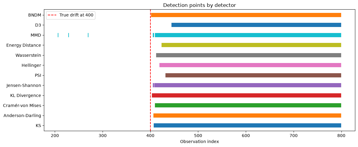
Visualising detection points#
We can compare how quickly each family of detectors reacts to the drift.
all_results = {**results, **results_dist, **results_multi, **results_bndm}

fig, ax = plt.subplots(figsize=(12, 5))
names = list(all_results.keys())
for idx, (name, dets) in enumerate(all_results.items()):
    if dets:
        ax.scatter(dets, [idx] * len(dets), marker="|", s=100, linewidths=1.5)
    else:
        ax.scatter([], [])

ax.axvline(half, color="red", linestyle="--", label=f"True drift at {half}")
ax.set_yticks(range(len(names)))
ax.set_yticklabels(names)
ax.set_xlabel("Observation index")
ax.set_title("Detection points by detector")
ax.legend()
plt.tight_layout()
plt.show()
6. Categorical features with Chi-Square#
The ChiSquare detector is designed for categorical (discrete) data.
It builds a contingency table per feature and applies the chi-square test
of independence.
from capymoa.drift.detectors import ChiSquare

categories = ["a", "b", "c"]
cat_ref = rng.choice(categories, size=(N_REF, 2), p=[0.5, 0.3, 0.2])
cat_stream = np.vstack(
    [
        rng.choice(categories, size=(half, 2), p=[0.5, 0.3, 0.2]),
        rng.choice(categories, size=(half, 2), p=[0.1, 0.2, 0.7]),
    ]
)

chi2 = ChiSquare(window_size=WINDOW)
chi2.fit(cat_ref)

chi2_dets = []
for i, x in enumerate(cat_stream):
    chi2.add_element(x)
    if chi2.detected_change():
        chi2_dets.append(i)

print(
    f"Chi-Square: first detection at {chi2_dets[0] if chi2_dets else 'N/A'} "
    f"(total {len(chi2_dets)} detections)"
)
Chi-Square: first detection at 418 (total 382 detections)
7. Batch comparison with compare()#
If you already have a test window, you can compare it against the
reference in one call. This skips the streaming loop and returns a
DataDriftResult directly.
from capymoa.drift.detectors import MMD, KolmogorovSmirnov

X_no_drift = rng.normal(0, 1, size=(WINDOW, N_FEATURES))
X_drifted = rng.normal(SHIFT, 1, size=(WINDOW, N_FEATURES))

for label, DetCls, kwargs in [
    ("KS", KolmogorovSmirnov, {"window_size": WINDOW}),
    ("MMD", MMD, {"window_size": WINDOW, "n_permutations": 50, "sigma": 1.0}),
]:
    det = DetCls(**kwargs)
    det.fit(X_ref)

    r_same = det.compare(X_no_drift)
    r_drift = det.compare(X_drifted)

    print(f"\n{label}:")
    print(f"  Same distribution → drift={r_same.is_drift}, stat={r_same.statistic:.4f}")
    print(
        f"  Shifted           → drift={r_drift.is_drift}, stat={r_drift.statistic:.4f}"
    )
KS:
  Same distribution → drift=False, stat=0.1180
  Shifted           → drift=True, stat=0.9120

MMD:
  Same distribution → drift=False, stat=-0.0009
  Shifted           → drift=True, stat=0.6748
8. Auto-fit mode#
If you do not have a separate reference dataset, you can let the detector
collect the first N observations as its reference by setting
auto_fit_samples. No explicit fit() call is needed; REQUIRES_FIT
stays True because a reference is still collected through add_element.
from capymoa.drift.detectors import KolmogorovSmirnov

ks_auto = KolmogorovSmirnov(window_size=WINDOW, auto_fit_samples=N_REF)

# Stream everything – the first N_REF samples are used as reference
all_data = np.vstack([X_ref, X_stream])
auto_dets = []
for i, x in enumerate(all_data):
    ks_auto.add_element(x)
    if ks_auto.detected_change():
        auto_dets.append(i)

# Drift is at N_REF + half
true_drift = N_REF + half
print(f"Auto-fit KS: first detection at {auto_dets[0] if auto_dets else 'N/A'}")
print(f"(True drift at observation {true_drift})")
Auto-fit KS: first detection at 908
(True drift at observation 900)
9. Feature names from pandas DataFrames#
When you pass a DataFrame to fit(), the detector extracts column names
automatically. These appear in the feature_names attribute.
df_ref = pd.DataFrame(X_ref, columns=["temperature", "humidity"])

ks_df = KolmogorovSmirnov(window_size=WINDOW)
ks_df.fit(df_ref)

print(f"Feature names: {ks_df.feature_names}")

result = ks_df.compare(X_stream[half : half + WINDOW])
print(f"Per-feature drift: {result.feature_is_drift}")
Feature names: ['temperature', 'humidity']
Per-feature drift: {'temperature': np.True_, 'humidity': np.True_}
Summary#
Category |
Detectors |
Data type |
|---|---|---|
Statistical tests |
KolmogorovSmirnov, AndersonDarling, CramerVonMises |
Numeric (univariate per feature) |
Distance-based |
KLDivergence, JensenShannon, PSI, Hellinger, Wasserstein, EnergyDistance |
Numeric (univariate per feature) |
Multivariate |
MMD, D3 |
Numeric (full feature vector) |
Bayesian |
BNDM |
Numeric (univariate per feature) |
Categorical |
ChiSquare |
Categorical |
All detectors share the same API. They have REQUIRES_FIT = True:
provide a reference with fit(X_ref), or set auto_fit_samples so
add_element collects it.
fit(X_ref)– set the reference distribution (not needed withauto_fit_samples).add_element(x)– stream a single observation.detected_change()– check if drift was detected.compare(X_test)– batch comparison returning aDataDriftResult(needsfit()).reset()– clear the sliding window (keeps reference).