
Optimizing Drift Detectors via Leave-One-Dataset-Out Cross-Validation#
Drift detectors have hyperparameters that control sensitivity. Defaults work well in some situations but poorly in others. This notebook shows a standardized protocol for tuning those hyperparameters:
Build several streams with known drift locations.
Train a classifier (Hoeffding Tree) on each stream, producing an error signal.
Run a candidate detector on each error signal and score it with
EvaluateDriftDetector.Use leave-one-dataset-out cross-validation: optimize on all but one dataset, then evaluate on the held-out one.
The evaluation metric is F1, which balances precision and recall of drift detections.
Reference: [1] Cerqueira, V., Gomes, H. M., Heyden, M., Pfahringer, B., & Bifet, A. (2026). A Framework for Evaluating and Benchmarking Concept Drift Detection Methods. ACM SIGKDD Conference on Knowledge Discovery and Data Mining.
More information about CapyMOA can be found at https://www.capymoa.org.
last update on 03/09/2026
import matplotlib.pyplot as plt
import numpy as np
import pandas as pd
from scipy.stats import randint, uniform
from sklearn.model_selection import ParameterSampler  # for random search

from capymoa.classifier import HoeffdingTree
from capymoa.drift.detectors import SEED
from capymoa.drift.eval_detector import EvaluateDriftDetector
from capymoa.evaluation import prequential_evaluation
from capymoa.stream.drift import AbruptDrift, Concept, DriftStream
from capymoa.stream.generator import (
    SEA,
    AgrawalGenerator,
    RandomTreeGenerator,
    STAGGERGenerator,
)
Benchmark Streams#
We create four synthetic streams as example, each with one abrupt drift. The streams use different generators so that the optimization is not tied to a single data source. Each stream contains 20 000 instances with a drift at instance 10 000. See reference [1] for realistic examples using real-world datasets with injected drifts.
MAX_INSTANCES = 20_000
DRIFT_AT = 10_000
MAX_DELAY = 500
N_SAMPLES = 20
RANDOM_STATE = 42
streams = {
    "SEA": DriftStream(
        stream=[
            Concept(SEA(function=1), num_instances=DRIFT_AT),
            AbruptDrift(),
            Concept(SEA(function=3), num_instances=DRIFT_AT),
        ]
    ),
    "STAGGER": DriftStream(
        stream=[
            Concept(
                STAGGERGenerator(classification_function=1),
                num_instances=DRIFT_AT,
            ),
            AbruptDrift(),
            Concept(
                STAGGERGenerator(classification_function=3),
                num_instances=DRIFT_AT,
            ),
        ]
    ),
    "RandomTree": DriftStream(
        stream=[
            Concept(RandomTreeGenerator(tree_random_seed=1), num_instances=DRIFT_AT),
            AbruptDrift(),
            Concept(RandomTreeGenerator(tree_random_seed=42), num_instances=DRIFT_AT),
        ]
    ),
    "Agrawal": DriftStream(
        stream=[
            Concept(
                AgrawalGenerator(classification_function=1, instance_random_seed=1),
                num_instances=DRIFT_AT,
            ),
            AbruptDrift(),
            Concept(
                AgrawalGenerator(classification_function=4, instance_random_seed=42),
                num_instances=DRIFT_AT,
            ),
        ]
    ),
}

for name, stream in streams.items():
    drifts = stream.get_drifts()
    positions = [d.position for d in drifts]
    print(f"{name:>12s}: drift(s) at {positions}")
         SEA: drift(s) at [10000]
     STAGGER: drift(s) at [10000]
  RandomTree: drift(s) at [10000]
     Agrawal: drift(s) at [10000]
Producing the Error Signal#
For each stream we run a Hoeffding Tree in the prequential (test-then-train) setting. We store the predictions and ground truth so that we can compute a binary error signal: 1 when the classifier is wrong, 0 when it is right. This error signal is what the drift detector will monitor.
def build_error_signal(stream, max_instances):
    """Run a Hoeffding Tree on `stream` and return a binary error signal."""
    learner = HoeffdingTree(schema=stream.get_schema())
    results = prequential_evaluation(
        stream,
        learner,
        max_instances=max_instances,
        store_predictions=True,
        store_y=True,
    )
    y_true = results.ground_truth_y()
    y_pred = results.predictions()
    errors = (y_true != y_pred).astype(float)
    return errors


error_signals = {}
for name, stream in streams.items():
    error_signals[name] = build_error_signal(stream, MAX_INSTANCES)
    print(
        f"{name:>12s}: {len(error_signals[name])} instances, "
        f"error rate = {error_signals[name].mean():.3f}"
    )
SEA: 20000 instances, error rate = 0.132
STAGGER: 20000 instances, error rate = 0.027
RandomTree: 20000 instances, error rate = 0.301
Agrawal: 20000 instances, error rate = 0.196
Defining the Optimization Search Space#
We use SEED (Streaming Ensemble Algorithm for Drift detection) as the example detector. It has several key parameters:
delta: significance level for the statistical test (default 0.05)block_size: size of data blocks for compression (default 32)epsilon_prime: tolerance parameter for drift detection (default 0.01)
Lower delta and epsilon_prime values make the detector more sensitive
(more alarms); higher block_size gives smoother but slower detection.
We use sklearn’s ParameterSampler for random search over both continuous
and discrete distributions.
param_distributions = {
    "delta": uniform(loc=0.01, scale=0.19),
    "block_size": randint(32, 65),
    "epsilon_prime": np.linspace(0.0025, 0.01, 11),
}

sampler = ParameterSampler(
    param_distributions, n_iter=N_SAMPLES, random_state=RANDOM_STATE
)
param_configs = list(sampler)

# Show a few sampled configurations
print(f"Sampled {len(param_configs)} configurations:")
for i, cfg in enumerate(param_configs[:5]):
    print(
        f"  {i + 1}. delta={cfg['delta']:.4f}, "
        f"block_size={cfg['block_size']}, "
        f"epsilon_prime={cfg['epsilon_prime']:.4f}"
    )
print("  ...")
Sampled 20 configurations:
  1. delta=0.0449, block_size=60, epsilon_prime=0.0077
  2. delta=0.0396, block_size=52, epsilon_prime=0.0040
  3. delta=0.0210, block_size=54, epsilon_prime=0.0077
  4. delta=0.1337, block_size=55, epsilon_prime=0.0055
  5. delta=0.1472, block_size=33, epsilon_prime=0.0063
  ...
Scoring a Single Configuration#
Given an error signal, a set of true drift positions, and a candidate parameter configuration, we run SEED and compute the F1 score.
def run_detector(error_signal, params):
    """Run SEED with given parameters on an error signal and return the
    list of detection indices."""
    detector = SEED(
        delta=params["delta"],
        block_size=params["block_size"],
        epsilon_prime=params["epsilon_prime"],
    )
    for val in error_signal:
        detector.add_element(val)
    return detector.detection_index


def evaluate_detector(error_signal, true_positions, params, max_delay):
    """Run SEED with `params` and return the metrics."""
    preds = run_detector(error_signal, params)

    evaluator = EvaluateDriftDetector(max_delay=max_delay)
    metrics = evaluator.calc_performance(
        trues=np.array(true_positions),
        preds=preds,
        tot_n_instances=len(error_signal),
    )
    return metrics
Scoring All Configurations on Every Dataset#
Before doing the cross-validation split, we first evaluate every sampled configuration on every dataset so that the full table of results is available.
dataset_names = list(streams.keys())

# Build a dict: scores[dataset_name][config_idx] = F1
scores = {}
for name in dataset_names:
    stream = streams[name]
    true_positions = [d.position for d in stream.get_drifts()]
    scores[name] = {}
    for idx, params in enumerate(param_configs):
        metrics = evaluate_detector(
            error_signals[name], true_positions, params, MAX_DELAY
        )
        scores[name][idx] = metrics.f1

# Create a DataFrame with config details as index
config_labels = [
    f"d={p['delta']:.3f}, bs={p['block_size']}, ep={p['epsilon_prime']:.4f}"
    for p in param_configs
]
scores_df = pd.DataFrame(scores)
scores_df.index = config_labels
scores_df.index.name = "config"
scores_df
| SEA | STAGGER | RandomTree | Agrawal | |
|---|---|---|---|---|
| config | ||||
| d=0.045, bs=60, ep=0.0077 | 0.000000 | 0.545455 | 0.285714 | 0.285714 |
| d=0.040, bs=52, ep=0.0040 | 0.000000 | 0.333333 | 0.444444 | 0.285714 |
| d=0.021, bs=54, ep=0.0077 | 0.000000 | 0.285714 | 0.285714 | 0.333333 |
| d=0.134, bs=55, ep=0.0055 | 0.285714 | 0.444444 | 0.285714 | 0.222222 |
| d=0.147, bs=33, ep=0.0063 | 0.250000 | 0.500000 | 0.285714 | 0.250000 |
| d=0.045, bs=33, ep=0.0055 | 0.000000 | 0.571429 | 0.285714 | 0.250000 |
| d=0.068, bs=64, ep=0.0063 | 0.000000 | 0.600000 | 0.250000 | 0.285714 |
| d=0.065, bs=56, ep=0.0100 | 0.000000 | 0.600000 | 0.285714 | 0.285714 |
| d=0.195, bs=59, ep=0.0040 | 0.200000 | 0.444444 | 0.250000 | 0.250000 |
| d=0.173, bs=34, ep=0.0070 | 0.250000 | 0.444444 | 0.250000 | 0.222222 |
| d=0.096, bs=52, ep=0.0033 | 0.000000 | 0.600000 | 0.285714 | 0.285714 |
| d=0.189, bs=35, ep=0.0033 | 0.250000 | 0.600000 | 0.250000 | 0.222222 |
| d=0.013, bs=40, ep=0.0033 | 0.000000 | 0.500000 | 0.285714 | 0.333333 |
| d=0.056, bs=51, ep=0.0070 | 0.333333 | 0.333333 | 0.285714 | 0.285714 |
| d=0.017, bs=39, ep=0.0025 | 0.000000 | 0.400000 | 0.285714 | 0.333333 |
| d=0.069, bs=35, ep=0.0063 | 0.000000 | 0.600000 | 0.285714 | 0.333333 |
| d=0.045, bs=35, ep=0.0033 | 0.000000 | 0.600000 | 0.444444 | 0.285714 |
| d=0.095, bs=57, ep=0.0092 | 0.333333 | 0.600000 | 0.285714 | 0.285714 |
| d=0.148, bs=45, ep=0.0077 | 0.250000 | 0.500000 | 0.250000 | 0.250000 |
| d=0.047, bs=45, ep=0.0085 | 0.000000 | 0.500000 | 0.285714 | 0.285714 |
Leave-One-Dataset-Out Cross-Validation#
For each held-out dataset:
Optimize: pick the configuration that maximizes the mean F1 over the remaining datasets.
Evaluate: apply that configuration to the held-out dataset and record the F1.
This simulates the real-world scenario where the detector is tuned on available data and then deployed on a new, unseen stream.
cv_results = []

for held_out in dataset_names:
    train_datasets = [d for d in dataset_names if d != held_out]

    # Mean F1 across training datasets for each config
    mean_f1_per_config = {}
    for idx in range(len(param_configs)):
        f1_values = [scores[d][idx] for d in train_datasets]
        mean_f1_per_config[idx] = np.mean(f1_values)

    # Best config on training datasets
    best_idx = max(mean_f1_per_config, key=mean_f1_per_config.get)
    best_params = param_configs[best_idx]
    best_train_f1 = mean_f1_per_config[best_idx]

    # Evaluate best config on the held-out dataset
    test_f1 = scores[held_out][best_idx]

    cv_results.append(
        {
            "held_out": held_out,
            "best_delta": round(best_params["delta"], 4),
            "best_block_size": best_params["block_size"],
            "best_epsilon_prime": round(best_params["epsilon_prime"], 4),
            "mean_train_f1": round(best_train_f1, 4),
            "test_f1": round(test_f1, 4),
            "_best_idx": best_idx,  # keep for later use
        }
    )

    print(
        f"Held out: {held_out:>12s} | "
        f"Best: delta={best_params['delta']:.4f}, bs={best_params['block_size']}, "
        f"ep={best_params['epsilon_prime']:.4f} | "
        f"Train F1 = {best_train_f1:.4f} | "
        f"Test F1 = {test_f1:.4f}"
    )

cv_df = pd.DataFrame(cv_results).drop(columns=["_best_idx"])
cv_df
Held out:          SEA | Best: delta=0.0451, bs=35, ep=0.0033 | Train F1 = 0.4434 | Test F1 = 0.0000
Held out:      STAGGER | Best: delta=0.0558, bs=51, ep=0.0070 | Train F1 = 0.3016 | Test F1 = 0.3333
Held out:   RandomTree | Best: delta=0.0955, bs=57, ep=0.0092 | Train F1 = 0.4063 | Test F1 = 0.2857
Held out:      Agrawal | Best: delta=0.0955, bs=57, ep=0.0092 | Train F1 = 0.4063 | Test F1 = 0.2857
| held_out | best_delta | best_block_size | best_epsilon_prime | mean_train_f1 | test_f1 | |
|---|---|---|---|---|---|---|
| 0 | SEA | 0.0451 | 35 | 0.0032 | 0.4434 | 0.0000 |
| 1 | STAGGER | 0.0558 | 51 | 0.0070 | 0.3016 | 0.3333 |
| 2 | RandomTree | 0.0955 | 57 | 0.0092 | 0.4063 | 0.2857 |
| 3 | Agrawal | 0.0955 | 57 | 0.0092 | 0.4063 | 0.2857 |
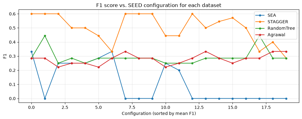
The plot below shows how F1 varies across sampled configurations for each dataset. Configurations are sorted by their mean F1 across all datasets.
# Sort configurations by mean F1 across datasets
mean_f1_per_config = [
    np.mean([scores[d][idx] for d in dataset_names])
    for idx in range(len(param_configs))
]
sorted_indices = np.argsort(mean_f1_per_config)[::-1]

fig, ax = plt.subplots(figsize=(10, 4))
for name in dataset_names:
    f1_values = [scores[name][idx] for idx in sorted_indices]
    ax.plot(range(len(param_configs)), f1_values, marker="o", markersize=4, label=name)

ax.set_xlabel("Configuration (sorted by mean F1)")
ax.set_ylabel("F1")
ax.set_title("F1 score vs. SEED configuration for each dataset")
ax.legend()
ax.grid(True, alpha=0.3)
plt.tight_layout()
plt.show()
Applying the Optimized Detector to a Held-Out Dataset#
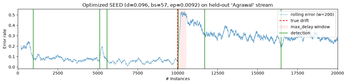
As a concrete example we pick the last fold – the one where Agrawal
was held out – and show the full detection trace on it.
# Use the last dataset as an example
example_fold = cv_results[-1]
held_out_name = example_fold["held_out"]
best_params = {
    "delta": example_fold["best_delta"],
    "block_size": example_fold["best_block_size"],
    "epsilon_prime": example_fold["best_epsilon_prime"],
}

print(f"Held-out dataset      : {held_out_name}")
print(f"Optimized delta       : {best_params['delta']:.4f}")
print(f"Optimized block_size  : {best_params['block_size']}")
print(f"Optimized epsilon_prime: {best_params['epsilon_prime']:.4f}")
print(f"Test F1               : {example_fold['test_f1']}")

# Run the optimized detector
detections = run_detector(error_signals[held_out_name], best_params)
true_positions = [d.position for d in streams[held_out_name].get_drifts()]

print(f"True drift(s)         : {true_positions}")
print(f"Detections            : {list(detections)}")
Held-out dataset      : Agrawal
Optimized delta       : 0.0955
Optimized block_size  : 57
Optimized epsilon_prime: 0.0092
Test F1               : 0.2857
True drift(s)         : [10000]
Detections            : [969, 5130, 5586, 10032, 11685, 16473]
fig, ax = plt.subplots(figsize=(12, 3))

# Rolling error rate for visual context
window = 200
rolling_error = pd.Series(error_signals[held_out_name]).rolling(window).mean()
ax.plot(rolling_error, linewidth=0.8, alpha=0.7, label=f"rolling error (w={window})")

# True drift locations
for i, pos in enumerate(true_positions):
    ax.axvline(
        pos,
        color="red",
        linestyle="--",
        linewidth=1.5,
        label="true drift" if i == 0 else None,
    )
    ax.axvspan(
        pos,
        pos + MAX_DELAY,
        color="red",
        alpha=0.08,
        label="max_delay window" if i == 0 else None,
    )

# Detections
for i, det in enumerate(detections):
    ax.axvline(
        det,
        color="green",
        linewidth=1.2,
        label="detection" if i == 0 else None,
    )

ax.set_xlim(0, MAX_INSTANCES)
ax.set_xlabel("# Instances")
ax.set_ylabel("Error rate")
ax.set_title(
    f"Optimized SEED (d={best_params['delta']:.3f}, bs={best_params['block_size']}, "
    f"ep={best_params['epsilon_prime']:.4f}) on held-out '{held_out_name}' stream"
)
ax.legend(loc="upper right")
plt.tight_layout()
plt.show()
Summary#
This notebook demonstrated a leave-one-dataset-out protocol for optimizing drift detector hyperparameters:
We built four synthetic streams with known drift locations.
A Hoeffding Tree produced a binary error signal on each stream.
We used sklearn’s
ParameterSamplerto randomly sample SEED configurations (delta,block_size, andepsilon_prime).We evaluated each configuration using the F1 metric from
EvaluateDriftDetector.For each held-out dataset, we selected the best configuration from the remaining three and measured how well it transferred.
The protocol generalizes to any detector and any set of hyperparameters. By evaluating on held-out data, the results give a more realistic estimate of how the tuned detector will perform on new streams.