
Automated machine learning#
This notebook contains some basics for autoML using CapyMOA:
Implement a custom model selection procedure using CapyMOA.
Perform hyperparameter optimisation, and model selection using CapyMOA’s AutoML features.
More information about CapyMOA can be found at https://www.capymoa.org.
last updated on 28/11/2025
import contextlib
import io

from moa.streams import ConceptDriftStream

from capymoa.automl import (
    AutoClass,
    BanditClassifier,
    EpsilonGreedy,
    SuccessiveHalvingClassifier,
)
from capymoa.classifier import (
    KNN,
    AdaptiveRandomForestClassifier,
    HoeffdingAdaptiveTree,
    HoeffdingTree,
    LeveragingBagging,
    NaiveBayes,
    StreamingRandomPatches,
)
from capymoa.datasets import Electricity
from capymoa.evaluation import prequential_evaluation
from capymoa.evaluation.visualization import plot_windowed_results
from capymoa.stream.drift import AbruptDrift, DriftStream, GradualDrift
from capymoa.stream.generator import SEA

# Setup the data streams for our experiments:
stream = Electricity()
drift_stream = DriftStream(
    moa_stream=ConceptDriftStream(),
    CLI="""
    -s (generators.AgrawalGenerator -f 1)
    -d (ConceptDriftStream
        -s (generators.AgrawalGenerator -f 2)
        -d (ConceptDriftStream -s (generators.AgrawalGenerator -f 3)
        -d (generators.AgrawalGenerator -f 4) -p 30000 -w 0)
        -p 20000 -w 0)
    -p 10000
    -w 0
""",
)
def print_summary(label: str, results):
    print(
        f"{label.ljust(10)} Cumulative accuracy = {results.accuracy():.2f}, "
        f"wall-clock time: {results.wallclock():.3f}"
    )
Custom model selection#
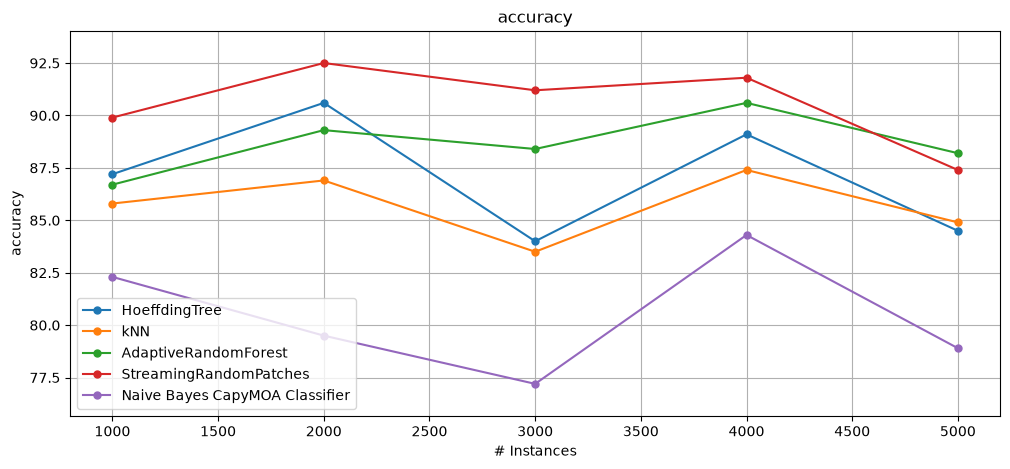
In this section we manually define a method to select the best model based on its accuracy on a given stream. First we define a list of models to be tried and then we iterate over the stream to train and evaluate each model. The model with the highest accuracy is selected as the best model.
# Define a generic adaptive learning function
def stream_learning_model_selection(model_list, window_size, max_instances):
    best_accuracy = 0  # The best accuracy score
    all_results = {}
    for model in model_list:
        results = prequential_evaluation(
            stream=stream,
            learner=model,
            window_size=window_size,
            max_instances=max_instances,
        )
        all_results[model] = results
        if results.cumulative.accuracy() > best_accuracy:
            best_accuracy = results.cumulative.accuracy()
            model_b = model

    print_summary(f"Best ({model_b})", all_results[model_b])
    return all_results
# Code to select the best performing model
schema = stream.get_schema()
ht = HoeffdingTree(schema)
knn = KNN(schema)
arf = AdaptiveRandomForestClassifier(schema, ensemble_size=5)
srp = StreamingRandomPatches(schema, ensemble_size=5)
nb = NaiveBayes(schema)
model_list = [ht, knn, arf, srp, nb]

all_res = stream_learning_model_selection(model_list, 1000, 5000)
plot_windowed_results(*all_res.values(), metric="accuracy")
Best (StreamingRandomPatches) Cumulative accuracy = 90.56, wall-clock time: 0.632
AutoML#
The following example shows how to use the AutoClass algorithm using CapyMOA.
base_classifiersis a list of classifier class types that will be candidates for the AutoML algorithm. The AutoML algorithm will select the best classifier based on its performance on the stream.configuration_jsonis a json file that contains the configuration for the AutoML algorithm. An example of the configuration file is shown below:
Maroua Bahri, Nikolaos Georgantas. Autoclass: Automl for data stream classification. In BigData, IEEE, 2023. https://ieeexplore.ieee.org/document/10386362
with open("./settings_autoclass.json", "r") as f:
    settings = f.read()
    print(settings)
{

  "windowSize" :  1000,
  "ensembleSize" : 10,
  "newConfigurations" : 10,
  "keepCurrentModel" : true,
  "lambda" : 0.05,
  "preventAlgorithmDeath" : true,
  "keepGlobalIncumbent" : true,
  "keepAlgorithmIncumbents" : true,
  "keepInitialConfigurations" : true,
  "useTestEnsemble" : true,
  "resetProbability" : 0.01,
  "numberOfCores" : 1,
  "performanceMeasureMaximisation": true,

  "algorithms": [
    {
      "algorithm": "moa.classifiers.lazy.kNN",
      "parameters": [
        {"parameter": "k", "type":"integer", "value":10, "range":[2,30]}
      ]
    }
  ,
    {
      "algorithm": "moa.classifiers.trees.HoeffdingTree",
      "parameters": [
        {"parameter": "g", "type":"integer", "value":200, "range":[10, 200]},
       {"parameter": "c", "type":"float", "value":0.01, "range":[0, 1]}
      ]
    }
  ,
    {
      "algorithm": "moa.classifiers.lazy.kNNwithPAWandADWIN",
      "parameters": [
        {"parameter": "k", "type":"integer", "value":10, "range":[2,30]}
      ]
    }
    ,
    {
      "algorithm": "moa.classifiers.trees.HoeffdingAdaptiveTree",
      "parameters": [
        {"parameter": "g", "type":"integer", "value":200, "range":[10, 200]},
        {"parameter": "c", "type":"float", "value":0.01, "range":[0, 1]}
      ]
    }

  ]
}
max_instances = 20000
window_size = 2500

schema = stream.get_schema()
autoclass = AutoClass(
    schema=schema,
    configuration_json="./settings_autoclass.json",
    base_classifiers=[KNN, HoeffdingAdaptiveTree, HoeffdingTree],
)
results_autoclass = prequential_evaluation(
    stream=stream,
    learner=autoclass,
    window_size=window_size,
    max_instances=max_instances,
)
print_summary("AutoClass", results_autoclass)
AutoClass Cumulative accuracy = 88.35, wall-clock time: 24.237
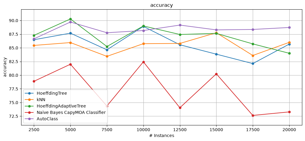
We compare the performance of the AutoML algorithm against basic classifiers:
ht = HoeffdingTree(schema)
hat = HoeffdingAdaptiveTree(schema)
knn = KNN(schema)
nb = NaiveBayes(schema)

results_ht = prequential_evaluation(
    stream, ht, window_size=window_size, max_instances=max_instances
)
results_hat = prequential_evaluation(
    stream, hat, window_size=window_size, max_instances=max_instances
)
results_knn = prequential_evaluation(
    stream, knn, window_size=window_size, max_instances=max_instances
)
results_nb = prequential_evaluation(
    stream, nb, window_size=window_size, max_instances=max_instances
)

print_summary("HT", results_ht)
print_summary("HAT", results_hat)
print_summary("KNN", results_knn)
print_summary("NB", results_nb)
plot_windowed_results(
    results_ht,
    results_knn,
    results_hat,
    results_nb,
    results_autoclass,
    metric="accuracy",
)
HT         Cumulative accuracy = 85.61, wall-clock time: 0.083
HAT        Cumulative accuracy = 87.08, wall-clock time: 0.157
KNN        Cumulative accuracy = 85.47, wall-clock time: 1.466
NB         Cumulative accuracy = 77.23, wall-clock time: 0.055
AutoML with concept drift#
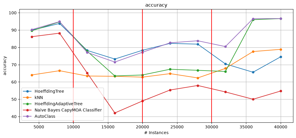
We test the same algorithms on a data stream with simulated concept drift:
from capymoa.automl import AutoClass
from capymoa.evaluation import prequential_evaluation

max_instances = 40000
window_size = 4000

ht = HoeffdingTree(schema=drift_stream.get_schema())
hat = HoeffdingAdaptiveTree(schema=drift_stream.get_schema())
knn = KNN(schema=drift_stream.get_schema())
nb = NaiveBayes(schema=drift_stream.get_schema())
autoclass = AutoClass(
    schema=drift_stream.get_schema(),
    configuration_json="./settings_autoclass.json",
    base_classifiers=[KNN, HoeffdingAdaptiveTree, HoeffdingTree],
)

results_ht = prequential_evaluation(
    drift_stream, ht, window_size=window_size, max_instances=max_instances
)
results_hat = prequential_evaluation(
    drift_stream, hat, window_size=window_size, max_instances=max_instances
)
results_knn = prequential_evaluation(
    drift_stream, knn, window_size=window_size, max_instances=max_instances
)
results_nb = prequential_evaluation(
    drift_stream, nb, window_size=window_size, max_instances=max_instances
)
results_autoclass = prequential_evaluation(
    drift_stream, autoclass, window_size=window_size, max_instances=max_instances
)

print_summary("HT", results_ht)
print_summary("HAT", results_hat)
print_summary("KNN", results_knn)
print_summary("NB", results_nb)
print_summary("AutoClass", results_autoclass)
plot_windowed_results(
    results_ht,
    results_knn,
    results_hat,
    results_nb,
    results_autoclass,
    metric="accuracy",
)
HT         Cumulative accuracy = 78.82, wall-clock time: 0.309
HAT        Cumulative accuracy = 78.24, wall-clock time: 0.349
KNN        Cumulative accuracy = 67.14, wall-clock time: 4.581
NB         Cumulative accuracy = 60.29, wall-clock time: 0.189
AutoClass  Cumulative accuracy = 85.10, wall-clock time: 73.102
Analysis of further AutoML methods#
Bandit Classifier#
It is a model selection for classification in streaming scenarios.
Each model is associated with an arm. At each train call, the policy decides which arm/model to pull. The reward is the performance of the model on the provided sample. The predict and predict_proba methods use the current best model.
Successive Halving Classifier#
The algorithm progressively eliminates poorly performing models while allocating more resources to promising ones.
Successive halving is a method for performing model selection without having to train each model on all the dataset. At certain points in time (called “rungs”), the worst performing models will be discarded and the best ones will keep competing between each other. The rung values are designed so that at most ‘budget’ model updates will be performed in total.
Testing whether SuccessiveHalvingClassifier and BanditClassifier work correctly#
f = io.StringIO()


def test_successive_halving_and_bandit(
    stream, max_instances=20000, window_size=2500, budget=None, bandit_eps=0.1
):
    """Test SuccessiveHalving and BanditClassifier for parameter optimization of a single model type."""
    print("\n" + "=" * 80)
    print("TESTING SUCCESSIVE HALVING AND BANDIT CLASSIFIER FOR PARAMETER OPTIMIZATION")
    print("=" * 80)

    schema = stream.get_schema()
    if budget is None:
        budget = max_instances * 2

    # Create a wide range of HoeffdingTree configurations with different parameters
    ht_models = []

    # Test different grace periods
    for grace_period in [50, 100, 200, 300, 400]:
        # Test different split confidences
        for confidence in [0.001, 0.01, 0.05, 0.1, 0.2]:
            # Test different tie thresholds
            for tie_threshold in [0.05, 0.1, 0.2]:
                ht_models.append(
                    HoeffdingTree(
                        schema=schema,
                        grace_period=grace_period,
                        confidence=confidence,
                        tie_threshold=tie_threshold,
                    )
                )

    print(f"Created {len(ht_models)} different HoeffdingTree configurations")

    # Use SuccessiveHalving to find the best HoeffdingTree configuration
    with contextlib.redirect_stdout(f):
        shc_ht = SuccessiveHalvingClassifier(
            schema=schema,
            base_classifiers=ht_models,
            budget=budget,
            eta=2.0,
            min_models=1,
            verbose=False,
        )

    # Use BanditClassifier to find the best HoeffdingTree configuration
    bandit_ht = BanditClassifier(
        schema=schema,
        base_classifiers=ht_models,
        metric="accuracy",
        policy=EpsilonGreedy(epsilon=bandit_eps, burn_in=150),
        verbose=False,
    )

    # Default HoeffdingTree for comparison
    default_ht = HoeffdingTree(schema=schema)

    print("\nRunning prequential evaluation...")
    results_shc_ht = prequential_evaluation(
        stream=stream,
        learner=shc_ht,
        window_size=window_size,
        max_instances=max_instances,
    )
    results_bandit_ht = prequential_evaluation(
        stream=stream,
        learner=bandit_ht,
        window_size=window_size,
        max_instances=max_instances,
    )
    results_default_ht = prequential_evaluation(
        stream=stream,
        learner=default_ht,
        window_size=window_size,
        max_instances=max_instances,
    )

    # Print results
    print("\nEvaluation Results:")
    print(
        f"[SuccessiveHalving with {len(ht_models)} HT configs] Accuracy = {results_shc_ht.accuracy():.3f}, "
        f"Time: {results_shc_ht.wallclock():.3f}s"
    )
    print(
        f"[BanditClassifier with {len(ht_models)} HT configs] Accuracy = {results_bandit_ht.accuracy():.3f}, "
        f"Time: {results_bandit_ht.wallclock():.3f}s"
    )
    print(
        f"[Default HoeffdingTree] Accuracy = {results_default_ht.accuracy():.3f}, "
        f"Time: {results_default_ht.wallclock():.3f}s"
    )

    # Calculate improvements
    improvement_shc = results_shc_ht.accuracy() - results_default_ht.accuracy()
    improvement_bandit = results_bandit_ht.accuracy() - results_default_ht.accuracy()
    print("Improvement over default parameters:")
    print(f"SuccessiveHalving: {improvement_shc:.2f}% absolute")
    print(f"BanditClassifier: {improvement_bandit:.2f}% absolute")

    # Plot results
    plot_windowed_results(
        results_shc_ht, results_bandit_ht, results_default_ht, metric="accuracy"
    )

    # Display final model info
    model_info_shc = shc_ht.get_model_info()
    print("\nSuccessive Halving Final Status:")
    print(
        f"Active models: {model_info_shc['active_models']} / {model_info_shc['total_models']}"
    )
    print(f"Total rungs: {model_info_shc['current_rung']}")
    print(
        f"Budget used: {model_info_shc['budget_used']} / {model_info_shc['total_budget']}"
    )
stream = Electricity()
max_instances = 20000
window_size = 2500
budget = max_instances * 2

test_successive_halving_and_bandit(
    stream, max_instances=max_instances, window_size=window_size, budget=budget
)
================================================================================
TESTING SUCCESSIVE HALVING AND BANDIT CLASSIFIER FOR PARAMETER OPTIMIZATION
================================================================================
Created 75 different HoeffdingTree configurations

Running prequential evaluation...
Evaluation Results:
[SuccessiveHalving with 75 HT configs] Accuracy = 87.225, Time: 132.661s
[BanditClassifier with 75 HT configs] Accuracy = 84.555, Time: 78.409s
[Default HoeffdingTree] Accuracy = 85.615, Time: 0.083s
Improvement over default parameters:
SuccessiveHalving: 1.61% absolute
BanditClassifier: -1.06% absolute
Successive Halving Final Status:
Active models: 1 / 75
Total rungs: 7
Budget used: 39999 / 40000
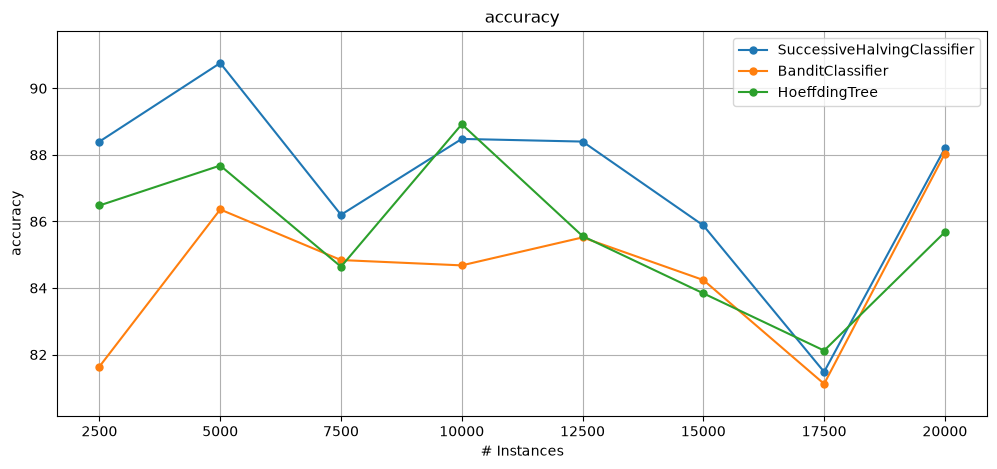
In the initial test, SuccessiveHalvingClassifier delivers the best accuracy (87.2%, +1.6% over HoeffdingTree) but takes 140s, while BanditClassifier is much faster (81s) with similar accuracy to the default, trading precision for speed.
The results highlight a clear accuracy–time trade-off between thorough configuration search and faster, less precise optimization.
Comparing AutoClass with SuccessiveHalving and BanditClassifier#
def base_models_configuration():
    # Create base classifiers with same parameters for SuccessiveHalving and BanditClassifier
    base_models = []

    # Add Hoeffding Trees
    for grace_period in [100, 200]:
        for confidence in [0.001, 0.01]:
            base_models.append(
                HoeffdingTree(
                    schema=schema, grace_period=grace_period, confidence=confidence
                )
            )

    # Add KNN variations
    for k in [3, 5]:
        base_models.append(KNN(schema=schema, k=k))

    # Add Random Forest models
    for ensemble_size in [60, 80]:
        base_models.append(
            AdaptiveRandomForestClassifier(schema=schema, ensemble_size=ensemble_size)
        )

    # Add Hoeffding Adaptive Trees
    for grace_period in [100, 200]:
        base_models.append(
            HoeffdingAdaptiveTree(schema=schema, grace_period=grace_period)
        )

    # Add Leveraging Bagging models
    for ensemble_size in [60, 80]:
        base_models.append(
            LeveragingBagging(schema=schema, ensemble_size=ensemble_size)
        )

    # Add Streaming Random Patches
    for ensemble_size in [60, 80]:
        base_models.append(
            StreamingRandomPatches(schema=schema, ensemble_size=ensemble_size)
        )

    return base_models
def autoclass(stream, max_instances, window_size, budget):
    schema = stream.get_schema()
    if budget is None:
        budget = max_instances * 3

    # Initialize AutoClass with the enhanced configuration
    autoclass_enhanced = AutoClass(
        schema=schema,
        configuration_json="./enhanced_autoclass_config.json",
        base_classifiers=[
            KNN,
            HoeffdingTree,
            HoeffdingAdaptiveTree,
            AdaptiveRandomForestClassifier,
            LeveragingBagging,
            StreamingRandomPatches,
        ],
    )

    results_autoclass_enhanced = prequential_evaluation(
        stream=stream,
        learner=autoclass_enhanced,
        window_size=window_size,
        max_instances=max_instances,
    )

    return results_autoclass_enhanced


def successive_halving(stream, max_instances, window_size):
    # Create base classifiers with same parameters for SuccessiveHalving and BanditClassifier
    base_models = base_models_configuration()

    # Create the SuccessiveHalvingClassifier
    with contextlib.redirect_stdout(f):
        shc_direct = SuccessiveHalvingClassifier(
            schema=schema,
            base_classifiers=base_models,
            budget=budget,
            eta=2.0,
            min_models=2,
            verbose=True,
        )

    results_shc = prequential_evaluation(
        stream=stream,
        learner=shc_direct,
        window_size=window_size,
        max_instances=max_instances,
    )

    return shc_direct, results_shc


def bandit_classifier(stream, max_instances, window_size, bandit_eps):
    # Create base classifiers with same parameters for SuccessiveHalving and BanditClassifier
    base_models = base_models_configuration()

    # Create the BanditClassifier
    bandit_clf = BanditClassifier(
        schema=schema,
        base_classifiers=base_models,
        metric="accuracy",
        policy=EpsilonGreedy(epsilon=bandit_eps, burn_in=150),
        verbose=True,
    )

    results_bandit = prequential_evaluation(
        stream=stream,
        learner=bandit_clf,
        window_size=window_size,
        max_instances=max_instances,
    )

    return bandit_clf, results_bandit
def test_autoclass_vs_successive_halving_and_bandit(
    stream,
    results_autoclass_enhanced,
    shc_direct,
    results_shc,
    bandit_clf,
    results_bandit,
    max_instances=20000,
    window_size=2500,
):
    """Compare AutoClass with enhanced configuration against SuccessiveHalvingClassifier and BanditClassifier."""
    print("\n" + "=" * 80)
    print("COMPARING AUTOCLASS WITH CONFIG, SUCCESSIVE HALVING, AND BANDIT CLASSIFIER")
    print("=" * 80)

    # Initialize default models for comparison
    print("\nInitializing default models for comparison...")
    default_ht = HoeffdingTree(schema=schema)
    default_knn = KNN(schema=schema)
    default_arf = AdaptiveRandomForestClassifier(schema=schema)
    default_hat = HoeffdingAdaptiveTree(schema=schema)
    default_lb = LeveragingBagging(schema=schema)
    default_srp = StreamingRandomPatches(schema=schema)

    # Evaluate default models
    print("\nEvaluating default models...")
    results_ht = prequential_evaluation(
        stream=stream,
        learner=default_ht,
        window_size=window_size,
        max_instances=max_instances,
    )
    results_knn = prequential_evaluation(
        stream=stream,
        learner=default_knn,
        window_size=window_size,
        max_instances=max_instances,
    )
    results_arf = prequential_evaluation(
        stream=stream,
        learner=default_arf,
        window_size=window_size,
        max_instances=max_instances,
    )
    results_hat = prequential_evaluation(
        stream=stream,
        learner=default_hat,
        window_size=window_size,
        max_instances=max_instances,
    )
    results_lb = prequential_evaluation(
        stream=stream,
        learner=default_lb,
        window_size=window_size,
        max_instances=max_instances,
    )
    results_srp = prequential_evaluation(
        stream=stream,
        learner=default_srp,
        window_size=window_size,
        max_instances=max_instances,
    )

    # Print results
    print("\nEvaluation Results:")
    print(
        f"[Enhanced AutoClass] Accuracy = {results_autoclass_enhanced.accuracy():.3f}, "
        f"Time: {results_autoclass_enhanced.wallclock():.3f}s"
    )
    print(
        f"[SuccessiveHalving] Accuracy = {results_shc.accuracy():.3f}, "
        f"Time: {results_shc.wallclock():.3f}s"
    )
    print(
        f"[BanditClassifier] Accuracy = {results_bandit.accuracy():.3f}, "
        f"Time: {results_bandit.wallclock():.3f}s"
    )
    print(
        f"[Default HoeffdingTree] Accuracy = {results_ht.accuracy():.3f}, "
        f"Time: {results_ht.wallclock():.3f}s"
    )
    print(
        f"[Default KNN] Accuracy = {results_knn.accuracy():.3f}, "
        f"Time: {results_knn.wallclock():.3f}s"
    )
    print(
        f"[Default AdaptiveRandomForest] Accuracy = {results_arf.accuracy():.3f}, "
        f"Time: {results_arf.wallclock():.3f}s"
    )
    print(
        f"[Default HoeffdingAdaptiveTree] Accuracy = {results_hat.accuracy():.3f}, "
        f"Time: {results_hat.wallclock():.3f}s"
    )
    print(
        f"[Default LeveragingBagging] Accuracy = {results_lb.accuracy():.3f}, "
        f"Time: {results_lb.wallclock():.3f}s"
    )
    print(
        f"[Default StreamingRandomPatches] Accuracy = {results_srp.accuracy():.3f}, "
        f"Time: {results_srp.wallclock():.3f}s"
    )

    # Plot results
    plot_windowed_results(
        results_autoclass_enhanced,
        results_shc,
        results_bandit,
        results_ht,
        results_knn,
        results_arf,
        results_hat,
        results_lb,
        results_srp,
        metric="accuracy",
    )

    # Display final model info for SuccessiveHalving
    model_info_shc = shc_direct.get_model_info()
    print("\nSuccessive Halving Final Status:")
    print(
        f"Active models: {model_info_shc['active_models']} / {model_info_shc['total_models']}"
    )
    print(f"Total rungs: {model_info_shc['current_rung']}")
    print(
        f"Budget used: {model_info_shc['budget_used']} / {model_info_shc['total_budget']}"
    )

    # Display final model info for BanditClassifier
    model_info_bandit = bandit_clf.get_model_info()
    print("\nBandit Classifier Final Status:")
    print(f"Total models: {model_info_bandit['total_models']}")
    print(f"Best model accuracy: {model_info_bandit['best_model_accuracy']:.4f}")

    print("\nTop performing models:")
    print("SuccessiveHalving:")
    for i, model_info in enumerate(model_info_shc["top_models"]):
        print(
            f"  {i + 1}. {model_info['model']} - Accuracy: {model_info['accuracy']:.4f}"
        )
Test on Electricity Stream#
stream = Electricity()
max_instances = 8000
window_size = 2000
budget = max_instances
results_autoclass = autoclass(
    stream, window_size=window_size, max_instances=max_instances, budget=budget
)
shc_direct, results_shc = successive_halving(stream, max_instances, window_size)
[Rung 1]	7 models removed	7 models left	142 instances per model	budget used: 1988	budget left: 6012	best accuracy: 95.0704
Top models:
  1. StreamingRandomPatches - Accuracy: 95.0704
  2. StreamingRandomPatches - Accuracy: 95.0704
  3. Leveraging OnlineBagging - Accuracy: 93.6620
[Rung 2]	3 models removed	4 models left	286 instances per model	budget used: 3990	budget left: 4010	best accuracy: 88.3178
Top models:
  1. StreamingRandomPatches - Accuracy: 88.3178
  2. StreamingRandomPatches - Accuracy: 88.3178
  3. Leveraging OnlineBagging - Accuracy: 87.3832
[Rung 3]	2 models removed	2 models left	501 instances per model	budget used: 5994	budget left: 2006	best accuracy: 90.9580
Top models:
  1. StreamingRandomPatches - Accuracy: 90.9580
  2. StreamingRandomPatches - Accuracy: 90.6351
bandit_clf, results_bandit = bandit_classifier(
    stream, max_instances, window_size, bandit_eps=0.3
)
Using 14 provided base classifiers
Chosen model: StreamingRandomPatches
Current accuracy: 90.7145
test_autoclass_vs_successive_halving_and_bandit(
    stream,
    window_size=window_size,
    max_instances=max_instances,
    results_autoclass_enhanced=results_autoclass,
    shc_direct=shc_direct,
    results_shc=results_shc,
    bandit_clf=bandit_clf,
    results_bandit=results_bandit,
)
================================================================================
COMPARING AUTOCLASS WITH CONFIG, SUCCESSIVE HALVING, AND BANDIT CLASSIFIER
================================================================================

Initializing default models for comparison...

Evaluating default models...
Evaluation Results:
[Enhanced AutoClass] Accuracy = 91.425, Time: 70.704s
[SuccessiveHalving] Accuracy = 91.300, Time: 68.928s
[BanditClassifier] Accuracy = 89.925, Time: 35.776s
[Default HoeffdingTree] Accuracy = 86.462, Time: 0.029s
[Default KNN] Accuracy = 84.775, Time: 0.559s
[Default AdaptiveRandomForest] Accuracy = 90.112, Time: 11.219s
[Default HoeffdingAdaptiveTree] Accuracy = 87.525, Time: 0.051s
[Default LeveragingBagging] Accuracy = 90.188, Time: 4.467s
[Default StreamingRandomPatches] Accuracy = 91.325, Time: 12.048s

Successive Halving Final Status:
Active models: 2 / 14
Total rungs: 3
Budget used: 5994 / 8000
Bandit Classifier Final Status:
Total models: 14
Best model accuracy: 90.2970

Top performing models:
SuccessiveHalving:
  1. StreamingRandomPatches - Accuracy: 91.5125
  2. StreamingRandomPatches - Accuracy: 91.4375
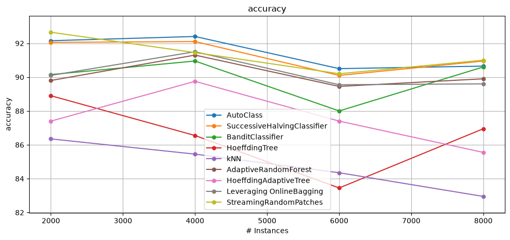
On Electricity, AutoClass achieves the highest accuracy (91.6%) but is slowest (134s).
SuccessiveHalvingClassifier nearly matches it (91.3%) while running faster, offering the best balance.
BanditClassifier (82.1%, 36s) is fastest but underperforms, even below the default HoeffdingTree (86.5%).
Overall, thorough model selection proves more effective here, with SuccessiveHalving striking the optimal trade-off.
Test on custom stream with drift#
window_size = 500
max_instances = 8000
budget = max_instances * 3
drift_stream = DriftStream(
    stream=[
        SEA(function=1),
        AbruptDrift(position=3000),
        SEA(function=3),
        GradualDrift(position=6000, width=2000),
        SEA(function=1),
    ]
)
results_autoclass = autoclass(
    drift_stream, window_size=window_size, max_instances=max_instances, budget=budget
)
shc_direct, results_shc = successive_halving(drift_stream, max_instances, window_size)
[Rung 1]	7 models removed	7 models left	428 instances per model	budget used: 5992	budget left: 18008	best accuracy: 80.8411
Top models:
  1. HoeffdingAdaptiveTree - Accuracy: 80.8411
  2. HoeffdingAdaptiveTree - Accuracy: 80.8411
  3. kNN - Accuracy: 80.3738
[Rung 2]	3 models removed	4 models left	857 instances per model	budget used: 11991	budget left: 12009	best accuracy: 85.9922
Top models:
  1. AdaptiveRandomForest - Accuracy: 85.9922
  2. kNN - Accuracy: 84.8249
  3. HoeffdingTree - Accuracy: 84.5914
[Rung 3]	2 models removed	2 models left	1501 instances per model	budget used: 17995	budget left: 6005	best accuracy: 87.2936
Top models:
  1. AdaptiveRandomForest - Accuracy: 87.2936
  2. Leveraging OnlineBagging - Accuracy: 85.9296
bandit_clf, results_bandit = bandit_classifier(
    drift_stream, max_instances, window_size, bandit_eps=0.3
)
Using 14 provided base classifiers
Chosen model: kNN
Current accuracy: 85.0684
test_autoclass_vs_successive_halving_and_bandit(
    drift_stream,
    window_size=window_size,
    max_instances=max_instances,
    results_autoclass_enhanced=results_autoclass,
    shc_direct=shc_direct,
    results_shc=results_shc,
    bandit_clf=bandit_clf,
    results_bandit=results_bandit,
)
================================================================================
COMPARING AUTOCLASS WITH CONFIG, SUCCESSIVE HALVING, AND BANDIT CLASSIFIER
================================================================================

Initializing default models for comparison...

Evaluating default models...
Evaluation Results:
[Enhanced AutoClass] Accuracy = 87.087, Time: 34.469s
[SuccessiveHalving] Accuracy = 86.775, Time: 72.587s
[BanditClassifier] Accuracy = 85.400, Time: 30.074s
[Default HoeffdingTree] Accuracy = 85.088, Time: 0.266s
[Default KNN] Accuracy = 84.362, Time: 0.673s
[Default AdaptiveRandomForest] Accuracy = 86.913, Time: 5.019s
[Default HoeffdingAdaptiveTree] Accuracy = 84.800, Time: 0.278s
[Default LeveragingBagging] Accuracy = 86.375, Time: 2.088s
[Default StreamingRandomPatches] Accuracy = 86.638, Time: 5.395s
Successive Halving Final Status:
Active models: 2 / 14
Total rungs: 3
Budget used: 17995 / 24000

Bandit Classifier Final Status:
Total models: 14
Best model accuracy: 85.5615

Top performing models:
SuccessiveHalving:
  1. AdaptiveRandomForest - Accuracy: 86.8750
  2. Leveraging OnlineBagging - Accuracy: 86.6000
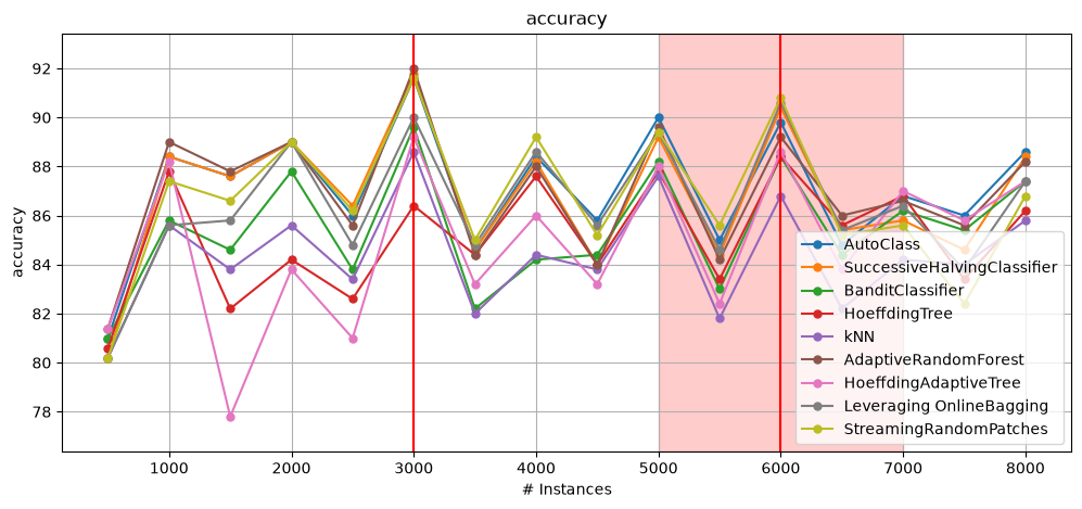
On the drift stream, Enhanced AutoClass reaches the top accuracy (86.9%) with moderate runtime (68s). BanditClassifier (85.2%, 37s) offers the best efficiency-accuracy balance, being more than 2x faster than SuccessiveHalving while losing only 1.4% accuracy.
AdaptiveRandomForest (86.7%) confirms that strong default ensembles can rival AutoML methods.
Overall Analysis#
Across tested streams, the three model selection approaches show consistent accuracy–efficiency trade-offs:
AutoClass: highest (or near-highest) accuracy, especially under concept drift, but slower than BanditClassifier.
SuccessiveHalvingClassifier: accuracy almost the one of AutoClass, but faster.
BanditClassifier: fastest but less accurate.
Guidelines based on these results:
Max accuracy & high resources → AutoClass.
Balance accuracy/efficiency → SuccessiveHalvingClassifier.
Time/resource-constrained → BanditClassifier.