Using PyTorch with CapyMOA#
This notebook demonstrates how use PyTorch with CapyMOA.
It contains examples showing:
How to define a PyTorch Network to be used with CapyMOA.
How a simple PyTorch model can be used in a CapyMOA
Instanceloop.How to define a PyTorch CapyMOA Classifier based on CapyMOA
Classifierframework and how to use it withprequential_evaluation().How to use a PyTorch dataset with a CapyMOA classifier.
Exploring Advanced Features(notebooks/common/advanced_API.py) includes an example using TensorBoard and aPyTorchClassifier.
More information about CapyMOA can be found at https://www.capymoa.org.
last update on 28/11/2025
Setup#
Sets random seed for reproducibility.
Sets PyTorch network .
Set random seeds#
import random

random_seed = 1
random.seed(random_seed)
Define network structure#
Here, the network uses the CPU device.
import torch
from torch import nn

torch.manual_seed(random_seed)
torch.use_deterministic_algorithms(True)

# Get cpu device for training.
device = "cpu"
print(f"Using {device} device")


# Define model
class NeuralNetwork(nn.Module):
    def __init__(self, input_size=0, number_of_classes=0):
        super().__init__()
        self.flatten = nn.Flatten()
        self.linear_relu_stack = nn.Sequential(
            nn.Linear(input_size, 512),
            nn.ReLU(),
            nn.Linear(512, 512),
            nn.ReLU(),
            nn.Linear(512, number_of_classes),
        )

    def forward(self, x):
        x = self.flatten(x)
        logits = self.linear_relu_stack(x)
        return logits
Using cpu device
Using an instance loop#
Model is initialised after receiving the first instance.
from capymoa.datasets import ElectricityTiny
from capymoa.evaluation import ClassificationEvaluator

elec_stream = ElectricityTiny()

# Creating the evaluator
evaluator = ClassificationEvaluator(schema=elec_stream.get_schema())

model = None
optimiser = None
loss_fn = nn.CrossEntropyLoss()

i = 0
while elec_stream.has_more_instances():
    i += 1
    instance = elec_stream.next_instance()
    if model is None:
        moa_instance = instance.java_instance.getData()
        # initialise the model and send it to the device
        model = NeuralNetwork(
            input_size=elec_stream.get_schema().get_num_attributes(),
            number_of_classes=elec_stream.get_schema().get_num_classes(),
        ).to(device)
        # set the optimiser
        optimiser = torch.optim.SGD(model.parameters(), lr=1e-3)
        print(model)

    X = torch.tensor(instance.x, dtype=torch.float32)
    y = torch.tensor(instance.y_index, dtype=torch.long)
    # set the device and add a dimension to the tensor
    X, y = torch.unsqueeze(X.to(device), 0), torch.unsqueeze(y.to(device), 0)

    # turn off gradient collection for test
    with torch.no_grad():
        pred = model(X)
        prediction = torch.argmax(pred)

    # update evaluator with predicted class
    evaluator.update(instance.y_index, prediction.item())

    # Compute prediction error
    pred = model(X)
    loss = loss_fn(pred, y)

    # Backpropagation
    loss.backward()
    optimiser.step()
    optimiser.zero_grad()

    if i % 500 == 0:
        print(f"Accuracy at {i} : {evaluator.accuracy()}")

print(f"Accuracy at {i} : {evaluator.accuracy()}")
NeuralNetwork(
  (flatten): Flatten(start_dim=1, end_dim=-1)
  (linear_relu_stack): Sequential(
    (0): Linear(in_features=6, out_features=512, bias=True)
    (1): ReLU()
    (2): Linear(in_features=512, out_features=512, bias=True)
    (3): ReLU()
    (4): Linear(in_features=512, out_features=2, bias=True)
  )
)
Accuracy at 500 : 50.4
Accuracy at 1000 : 55.2
Accuracy at 1500 : 61.199999999999996
Accuracy at 2000 : 61.1
Accuracy at 2000 : 61.1
PyTorchClassifier#
Defining a
PyTorchClassifierusing the CapyMOA API makes it compatible with CapyMOA functions likeprequential_evaluation()without losing the flexibility of specifying thearchitectureand thetrainingmethod.The model is initialised after receiving the first instance.
PyTorchClassifieris based on thecapymoa.baseClassifierabstract class.Important: We can access information about the stream through any of its instances. See
set_model(self, instance)for an example:
...
moa_instance = instance.java_instance.getData()
self.model = NeuralNetwork(input_size=moa_instance.get_num_attributes(),
                           number_of_classes=moa_instance.get_num_classes()).to(self.device)
...
import numpy as np

from capymoa.base import Classifier


class PyTorchClassifier(Classifier):
    def __init__(
        self,
        schema=None,
        random_seed=1,
        nn_model: nn.Module = None,
        optimiser=None,
        loss_fn=None,
        device=("cpu"),
        lr=1e-3,
    ):
        super().__init__(schema, random_seed)
        if loss_fn is None:
            loss_fn = nn.CrossEntropyLoss()
        self.model = None
        self.optimiser = None
        self.loss_fn = loss_fn
        self.lr = lr
        self.device = device

        torch.manual_seed(random_seed)

        if nn_model is None:
            self.set_model(None)
        else:
            self.model = nn_model.to(device)
        if optimiser is None:
            if self.model is not None:
                self.optimiser = torch.optim.SGD(self.model.parameters(), lr=lr)
        else:
            self.optimiser = optimiser

    def __str__(self):
        return str(self.model)

    def cli_help(self):
        return 'schema=None, random_seed=1, nn_model: nn.Module=None, optimiser=None, loss_fn=nn.CrossEntropyLoss(), device=("cpu"), lr=1e-3'

    def set_model(self, instance):
        if self.schema is None:
            moa_instance = instance.java_instance.getData()
            self.model = NeuralNetwork(
                input_size=moa_instance.get_num_attributes(),
                number_of_classes=moa_instance.get_num_classes(),
            ).to(self.device)
        elif instance is not None:
            self.model = NeuralNetwork(
                input_size=self.schema.get_num_attributes(),
                number_of_classes=self.schema.get_num_classes(),
            ).to(self.device)

    def train(self, instance):
        if self.model is None:
            self.set_model(instance)

        X = torch.tensor(instance.x, dtype=torch.float32)
        y = torch.tensor(instance.y_index, dtype=torch.long)
        # set the device and add a dimension to the tensor
        X, y = (
            torch.unsqueeze(X.to(self.device), 0),
            torch.unsqueeze(y.to(self.device), 0),
        )

        # Compute prediction error
        pred = self.model(X)
        loss = self.loss_fn(pred, y)

        # Backpropagation
        loss.backward()
        self.optimiser.step()
        self.optimiser.zero_grad()

    def predict(self, instance):
        return np.argmax(self.predict_proba(instance))

    def predict_proba(self, instance):
        if self.model is None:
            self.set_model(instance)
        X = torch.unsqueeze(
            torch.tensor(instance.x, dtype=torch.float32).to(self.device), 0
        )
        # turn off gradient collection
        with torch.no_grad():
            pred = np.asarray(self.model(X).numpy(), dtype=np.double)
        return pred
Using PyTorchClassifier + prequential_evaluation#
We can access information about the stream through the
schemadirectly, from the example below:
...
nn_model=NeuralNetwork(input_size=elec_stream.get_schema().get_num_attributes(),
                       number_of_classes=elec_stream.get_schema().get_num_classes()).to(device)
...
from capymoa.evaluation import prequential_evaluation

## Opening a file as a stream
elec_stream = ElectricityTiny()

# Creating a learner
simple_pyTorch_classifier = PyTorchClassifier(
    schema=elec_stream.get_schema(),
    nn_model=NeuralNetwork(
        input_size=elec_stream.get_schema().get_num_attributes(),
        number_of_classes=elec_stream.get_schema().get_num_classes(),
    ).to(device),
)

evaluator = prequential_evaluation(
    stream=elec_stream,
    learner=simple_pyTorch_classifier,
    window_size=4500,
    optimise=False,
)

print(f"Accuracy: {evaluator.cumulative.accuracy()}")
Accuracy: 62.849999999999994
How to use a PyTorch dataset with a CapyMOA classifier#
One may want to use various PyTorch datasets with different CapyMOA classifiers.
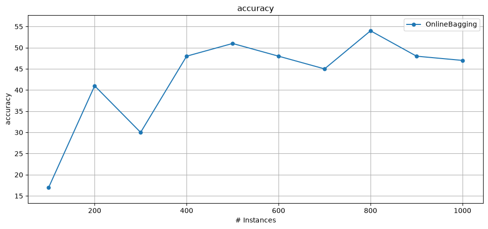
In this example we use PyTorch Dataset + prequential evaluation + CapyMOA Classifier.
Observation: Using a learner like Online Bagging without any feature extraction is not going to yield meaningful performance
from torchvision import datasets
from torchvision.transforms import ToTensor

from capymoa.classifier import OnlineBagging
from capymoa.evaluation import prequential_evaluation
from capymoa.evaluation.visualization import plot_windowed_results
from capymoa.stream import TorchStream

pytorch_dataset = datasets.FashionMNIST(
    root="data", train=True, download=True, transform=ToTensor()
)
pytorch_stream = TorchStream.from_classification(
    dataset=pytorch_dataset, num_classes=10
)

# Creating a learner
ob_learner = OnlineBagging(schema=pytorch_stream.get_schema(), ensemble_size=5)

results_ob_learner = prequential_evaluation(
    stream=pytorch_stream, learner=ob_learner, window_size=100, max_instances=1000
)

print(f"Accuracy: {results_ob_learner.cumulative.accuracy()}")
display(results_ob_learner.windowed.metrics_per_window())
plot_windowed_results(results_ob_learner, metric="accuracy")
0%| | 0.00/26.4M [00:00<?, ?B/s]
0%| | 32.8k/26.4M [00:00<01:25, 310kB/s]
0%| | 65.5k/26.4M [00:00<01:25, 308kB/s]
0%| | 131k/26.4M [00:00<00:58, 448kB/s]
1%| | 229k/26.4M [00:00<00:41, 634kB/s]
1%|▏ | 360k/26.4M [00:00<00:30, 847kB/s]
2%|▏ | 492k/26.4M [00:00<00:26, 975kB/s]
2%|▏ | 623k/26.4M [00:00<00:24, 1.06MB/s]
3%|▎ | 754k/26.4M [00:00<00:23, 1.11MB/s]
4%|▎ | 950k/26.4M [00:00<00:19, 1.34MB/s]
5%|▌ | 1.34M/26.4M [00:01<00:12, 2.05MB/s]
7%|▋ | 1.74M/26.4M [00:01<00:09, 2.54MB/s]
8%|▊ | 2.06M/26.4M [00:01<00:08, 2.71MB/s]
9%|▉ | 2.36M/26.4M [00:01<00:08, 2.72MB/s]
11%|█▏ | 3.01M/26.4M [00:01<00:06, 3.75MB/s]
14%|█▍ | 3.67M/26.4M [00:01<00:05, 4.47MB/s]
19%|█▉ | 5.05M/26.4M [00:01<00:03, 6.99MB/s]
24%|██▍ | 6.32M/26.4M [00:01<00:02, 8.48MB/s]
35%|███▍ | 9.18M/26.4M [00:01<00:01, 13.9MB/s]
46%|████▌ | 12.1M/26.4M [00:02<00:00, 17.8MB/s]
61%|██████▏ | 16.2M/26.4M [00:02<00:00, 23.7MB/s]
77%|███████▋ | 20.3M/26.4M [00:02<00:00, 27.9MB/s]
93%|█████████▎| 24.4M/26.4M [00:02<00:00, 30.8MB/s]
100%|██████████| 26.4M/26.4M [00:02<00:00, 11.2MB/s]
0%| | 0.00/29.5k [00:00<?, ?B/s]
100%|██████████| 29.5k/29.5k [00:00<00:00, 278kB/s]
100%|██████████| 29.5k/29.5k [00:00<00:00, 276kB/s]
0%| | 0.00/4.42M [00:00<?, ?B/s]
1%| | 32.8k/4.42M [00:00<00:13, 314kB/s]
1%|▏ | 65.5k/4.42M [00:00<00:13, 313kB/s]
2%|▏ | 98.3k/4.42M [00:00<00:13, 312kB/s]
4%|▍ | 197k/4.42M [00:00<00:07, 558kB/s]
7%|▋ | 295k/4.42M [00:00<00:05, 691kB/s]
10%|▉ | 426k/4.42M [00:00<00:04, 879kB/s]
13%|█▎ | 590k/4.42M [00:00<00:03, 1.10MB/s]
19%|█▉ | 852k/4.42M [00:00<00:02, 1.54MB/s]
25%|██▌ | 1.11M/4.42M [00:00<00:01, 1.84MB/s]
36%|███▋ | 1.61M/4.42M [00:01<00:01, 2.70MB/s]
47%|████▋ | 2.10M/4.42M [00:01<00:00, 3.31MB/s]
68%|██████▊ | 3.01M/4.42M [00:01<00:00, 4.95MB/s]
90%|█████████ | 4.00M/4.42M [00:01<00:00, 6.28MB/s]
100%|██████████| 4.42M/4.42M [00:01<00:00, 3.22MB/s]
0%| | 0.00/5.15k [00:00<?, ?B/s]
100%|██████████| 5.15k/5.15k [00:00<00:00, 17.8MB/s]
Accuracy: 42.9
| instances | accuracy | kappa | kappa_t | kappa_m | f1_score | F1 Score macro (percent) | f1_score_0 | f1_score_1 | f1_score_2 | ... | recall_1 | recall_2 | recall_3 | recall_4 | recall_5 | recall_6 | recall_7 | recall_8 | recall_9 | roc_auc | |
|---|---|---|---|---|---|---|---|---|---|---|---|---|---|---|---|---|---|---|---|---|---|
| 0 | 100.0 | 17.0 | 6.267645 | 0.000000 | 0.000000 | 17.0 | 14.458980 | 23.188406 | 30.769231 | 46.153846 | ... | 18.181818 | 33.333333 | 6.666667 | 0.000000 | 0.000000 | 0.000000 | 12.500000 | 0.000000 | 18.181818 | NaN |
| 1 | 200.0 | 41.0 | 33.288105 | 32.954545 | 30.588235 | 41.0 | 35.453087 | 39.130435 | 57.142857 | 36.363636 | ... | 40.000000 | 22.222222 | 0.000000 | 22.222222 | 22.222222 | 63.636364 | 23.076923 | 75.000000 | 12.500000 | NaN |
| 2 | 300.0 | 30.0 | 22.127044 | 23.076923 | 23.076923 | 30.0 | 32.728376 | 24.390244 | 72.727273 | 51.851852 | ... | 57.142857 | 53.846154 | 0.000000 | 9.090909 | 18.181818 | 33.333333 | 22.222222 | 18.181818 | 50.000000 | NaN |
| 3 | 400.0 | 48.0 | 41.775837 | 43.478261 | 42.222222 | 48.0 | 46.874041 | 36.363636 | 70.588235 | 22.222222 | ... | 54.545455 | 25.000000 | 8.333333 | 25.000000 | 66.666667 | 50.000000 | 63.636364 | 66.666667 | 33.333333 | NaN |
| 4 | 500.0 | 51.0 | 45.591828 | 45.555556 | 42.352941 | 51.0 | 50.423644 | 39.024390 | 50.000000 | 23.529412 | ... | 40.000000 | 16.666667 | 12.500000 | 50.000000 | 75.000000 | 25.000000 | 62.500000 | 78.571429 | 54.545455 | NaN |
| 5 | 600.0 | 48.0 | 42.164387 | 39.534884 | 36.585366 | 48.0 | 46.150940 | 38.888889 | 50.000000 | 47.058824 | ... | 33.333333 | 40.000000 | 0.000000 | 50.000000 | 71.428571 | 46.153846 | 50.000000 | 62.500000 | 61.538462 | NaN |
| 6 | 700.0 | 45.0 | 38.347719 | 35.294118 | 28.571429 | 45.0 | 43.987433 | 32.653061 | 80.000000 | 50.000000 | ... | 66.666667 | 57.142857 | 0.000000 | 61.538462 | 25.000000 | 33.333333 | 16.666667 | 68.750000 | 42.857143 | NaN |
| 7 | 800.0 | 54.0 | 48.221522 | 48.314607 | 45.882353 | 54.0 | 48.401026 | 44.444444 | 96.551724 | 60.000000 | ... | 93.333333 | 50.000000 | 0.000000 | 66.666667 | 53.846154 | 27.272727 | 10.000000 | 63.636364 | 37.500000 | NaN |
| 8 | 900.0 | 48.0 | 40.895658 | 43.478261 | 40.229885 | 48.0 | 44.715797 | 51.851852 | 81.818182 | 15.384615 | ... | 69.230769 | 16.666667 | 45.454545 | 16.666667 | 50.000000 | 33.333333 | 20.000000 | 44.444444 | 42.857143 | NaN |
| 9 | 1000.0 | 47.0 | 41.410568 | 44.791667 | 39.772727 | 47.0 | 45.810789 | 34.782609 | 85.714286 | 55.555556 | ... | 85.714286 | 50.000000 | 12.500000 | 75.000000 | 60.000000 | 27.272727 | 6.250000 | 87.500000 | 12.500000 | NaN |
10 rows × 42 columns