Exploring advanced features

This notebook is targeted at advanced users that want to access MOA objects directly using CapyMOA’s Python API.

In this notebook, we include:

• Examples on how to use any MOA classifier or regressor from CapyMOA.

• An example of how preprocessing (from MOA) can be used.

• Comparing a sklearn model to a MOA model.

• A variation of Creating a new classifier in CapyMOA (notebooks/classifier/new_learner.py) which uses MOA learners, thus accessing MOA (Java) objects directly.

• How to log experiments using TensorBoard alongside the PyTorch API. This extends Using PyTorch with CapyMOA (notebooks/common/pytorch_integration.py).

• Creating a synthetic stream with concept drifts using the MOA CLI directly.

• An example utilising a multi-threaded ensemble.

---

More information about CapyMOA can be found at https://www.capymoa.org.

last update on 06/08/2026

Using any MOA learner

• CapyMOA gives you access to any MOA classifier or regressor.

• For some MOA learners, there are corresponding Python objects (such as the HoeffdingTree or AdaptiveRandomForestClassifier). However, MOA has over a hundred learners, and more are added constantly.

• To allow advanced users to access any MOA learner from CapyMOA, we included the MOAClassifier and MOARegressor generic wrappers.

# This is an import from MOA
from moa.classifiers.trees import HoeffdingAdaptiveTree

from capymoa.base import MOAClassifier
from capymoa.datasets import Electricity
from capymoa.evaluation import prequential_evaluation

stream = Electricity()

# Creates a wrapper around the HoeffdingAdaptiveTree, which then can be used as any other CapyMOA classifier
HAT = MOAClassifier(schema=stream.get_schema(), moa_learner=HoeffdingAdaptiveTree)

results_HAT = prequential_evaluation(stream=stream, learner=HAT, window_size=500)

print(
    f"Cumulative accuracy = {results_HAT['cumulative'].accuracy()}, wall-clock time: {results_HAT['wallclock']}"
)
display(results_HAT["windowed"].metrics_per_window())

Cumulative accuracy = 83.38629943502825, wall-clock time: 0.8600263595581055

	instances	accuracy	kappa	kappa_t	kappa_m	f1_score	F1 Score macro (percent)	f1_score_0	f1_score_1	precision	Precision macro (percent)	precision_0	precision_1	recall	Recall macro (percent)	recall_0	recall_1	roc_auc
0	500.0	86.0	71.762808	-9.375000	68.888889	86.0	85.880492	84.581498	87.179487	86.0	85.939394	85.333333	86.545455	86.0	85.832836	83.842795	87.822878	0.905348
1	1000.0	89.2	78.456874	28.947368	78.988327	89.2	89.199309	89.285714	89.112903	89.2	89.408294	94.142259	84.674330	89.2	89.474107	84.905660	94.042553	0.937701
2	1500.0	95.8	86.827579	66.129032	83.064516	95.8	93.412757	89.447236	97.378277	95.8	94.263385	91.752577	96.774194	95.8	92.622426	87.254902	97.989950	0.950901
3	2000.0	77.0	54.896301	-47.435897	41.326531	77.0	76.911247	75.479744	78.342750	77.0	78.232560	64.835165	91.629956	77.0	79.363588	90.306122	68.421053	0.933047
4	2500.0	86.2	71.983109	25.000000	68.636364	86.2	85.991497	84.282460	87.700535	86.2	86.009685	84.474886	87.544484	86.2	85.974026	84.090909	87.857143	0.927850
...	...	...	...	...	...	...	...	...	...	...	...	...	...	...	...	...	...	...
86	43500.0	84.4	66.158171	20.408163	62.679426	84.4	82.620321	77.058824	88.181818	84.4	89.430894	100.000000	78.861789	84.4	81.339713	62.679426	100.000000	0.883610
87	44000.0	77.4	35.265811	-32.941176	28.481013	77.4	65.078404	44.334975	85.821832	77.4	87.582418	100.000000	75.164835	77.4	64.240506	28.481013	100.000000	0.882668
88	44500.0	72.0	39.008452	-105.882353	36.073059	72.0	66.916213	53.947368	79.885057	72.0	81.729270	96.470588	66.987952	72.0	68.187653	37.442922	98.932384	0.881889
89	45000.0	77.6	52.642706	-77.777778	45.365854	77.6	76.230900	70.526316	81.935484	77.6	77.362637	76.571429	78.153846	77.6	75.733774	65.365854	86.101695	0.881199
90	45312.0	76.4	52.842253	-38.823529	47.555556	76.4	76.336013	75.105485	77.566540	76.4	76.446493	70.634921	82.258065	76.4	76.780738	80.180180	73.381295	0.880594

91 rows × 18 columns

Checking the hyperparameters for the MOA CLI

• MOA objects can be parametrized using the MOA CLI (Command Line Interface)

• Sometimes you may not know the relevent parameters for a moa_learner, moa_learner.cli_help() presents all the hyperparameters available for the moa_learner object.

from moa.classifiers.meta import AdaptiveRandomForest

arf = MOAClassifier(schema=stream.get_schema(), moa_learner=AdaptiveRandomForest)

print(arf.cli_help())

-l treeLearner (default: ARFHoeffdingTree -e 2000000 -g 50 -c 0.01)
Random Forest Tree.
-s ensembleSize (default: 100)
The number of trees.
-o mFeaturesMode (default: Percentage (M * (m / 100)))
Defines how m, defined by mFeaturesPerTreeSize, is interpreted. M represents the total number of features.
-m mFeaturesPerTreeSize (default: 60)
Number of features allowed considered for each split. Negative values corresponds to M - m
-a lambda (default: 6.0)
The lambda parameter for bagging.
-j numberOfJobs (default: 1)
Total number of concurrent jobs used for processing (-1 = as much as possible, 0 = do not use multithreading)
-x driftDetectionMethod (default: ADWINChangeDetector -a 1.0E-3)
Change detector for drifts and its parameters
-p warningDetectionMethod (default: ADWINChangeDetector -a 1.0E-2)
Change detector for warnings (start training bkg learner)
-w disableWeightedVote
Should use weighted voting?
-u disableDriftDetection
Should use drift detection? If disabled then bkg learner is also disabled
-q disableBackgroundLearner
Should use bkg learner? If disabled then reset tree immediately.

Using preprocessing from MOA (filters)

We are working on a more user friendly API for preprocessing, this example just shows how one can do that using MOA filters from CapyMOA.

• Here we use NormalisationFilter filter from MOA to normalize instances in an online fashion.

• MOA filter syntax wraps the whole stream, so we are always composing commands like FilteredStream.

• We obtain the MOA CLI from the rbf_100k stream. Since it can be mapped to a MOA stream, it is possible to obtain it. Comment out the print statements below if you would like to inspect the actual creation strings (and perhaps try to copy and paste that into MOA).

from moa.streams import FilteredStream

from capymoa.classifier import OnlineBagging
from capymoa.datasets import Electricity, get_download_dir
from capymoa.evaluation import prequential_evaluation
from capymoa.stream import MOAStream

stream = Electricity()
elec_file = "electricity.arff"

cli = f"-s (ArffFileStream -f {get_download_dir() / elec_file}) -f NormalisationFilter"
print(cli)

# Create a FilterStream and use the NormalisationFilter
rbf_stream_normalised = MOAStream(CLI=cli, moa_stream=FilteredStream())

# print(f'MOA creation string for filtered version: {rbf_stream_normalised.moa_stream.getCLICreationString(rbf_stream_normalised.moa_stream.__class__)}')
ob_learner_norm = OnlineBagging(
    schema=rbf_stream_normalised.get_schema(), ensemble_size=5
)
ob_learner = OnlineBagging(schema=stream.get_schema(), ensemble_size=5)

ob_results_norm = prequential_evaluation(
    stream=rbf_stream_normalised, learner=ob_learner_norm
)
ob_results = prequential_evaluation(stream=stream, learner=ob_learner)

print(
    f"\tAccuracy with online normalisation: {ob_results_norm['cumulative'].accuracy()}"
)
print(f"\tAccuracy without normalisation: {ob_results['cumulative'].accuracy()}")

-s (ArffFileStream -f data/electricity.arff) -f NormalisationFilter

	Accuracy with online normalisation: 80.53937146892656
	Accuracy without normalisation: 82.06656073446328

Comparing a MOA and sklearn models

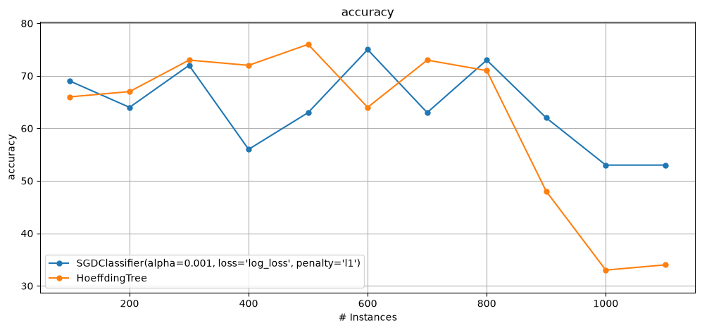
• This example shows how simple it is to compare MOA and sklearn regressors.

• We use wrappers for the sake of this example.

• SKClassifier (and SKRegressor) are parametrised directly as part of the object initialisation.

• MOAClassifier (and MOARegressor) are parametrised through a CLI (a separate parameter).

from moa.classifiers.trees import HoeffdingTree
from sklearn.linear_model import SGDClassifier

from capymoa.base import MOAClassifier, SKClassifier
from capymoa.datasets import CovtypeTiny
from capymoa.evaluation import prequential_evaluation_multiple_learners
from capymoa.evaluation.visualization import plot_windowed_results

covt_tiny = CovtypeTiny()

sk_sgd = SKClassifier(
    schema=covt_tiny.schema,
    sklearner=SGDClassifier(loss="log_loss", penalty="l1", alpha=0.001),
)
moa_ht = MOAClassifier(schema=covt_tiny.schema, moa_learner=HoeffdingTree, CLI="-g 50")

results = prequential_evaluation_multiple_learners(
    stream=covt_tiny, learners={"sk_sgd": sk_sgd, "moa_ht": moa_ht}, window_size=100
)
plot_windowed_results(results["sk_sgd"], results["moa_ht"], metric="accuracy")

Creating Python learners with MOA Objects

• This follows the example from new_learner which shows how to create a custom online bagging implementation.

• Here we also create an online bagging implementation, but the base_learner is a MOA class instead.

from collections import Counter

import numpy as np
from moa.classifiers.trees import HoeffdingTree

from capymoa.base import Classifier, MOAClassifier


class CustomOnlineBagging(Classifier):
    def __init__(
        self,
        schema=None,
        random_seed=1,
        ensemble_size=5,
        moa_base_learner_class=None,
        CLI_base_learner=None,
    ):
        super().__init__(schema=schema, random_seed=random_seed)

        self.CLI_base_learner = CLI_base_learner

        self.ensemble_size = ensemble_size
        self.moa_base_learner_class = moa_base_learner_class

        # Default base learner if None is specified
        if self.moa_base_learner_class is None:
            self.moa_base_learner_class = HoeffdingTree

        self.ensemble = []
        # Create several instances for the base_learners
        for _ in range(self.ensemble_size):
            self.ensemble.append(
                MOAClassifier(
                    schema=self.schema,
                    moa_learner=self.moa_base_learner_class(),
                    CLI=self.CLI_base_learner,
                )
            )

    def __str__(self):
        return "CustomOnlineBagging"

    def train(self, instance):
        for i in range(self.ensemble_size):
            for _ in range(np.random.poisson(1.0)):
                self.ensemble[i].train(instance)

    def predict(self, instance):
        predictions = []
        for i in range(self.ensemble_size):
            predictions.append(self.ensemble[i].predict(instance))
        majority_vote = Counter(predictions)
        prediction = majority_vote.most_common(1)[0][0]
        return prediction

    def predict_proba(self, instance):
        probabilities = []
        for i in range(self.ensemble_size):
            classifier_proba = self.ensemble[i].predict_proba(instance)
            classifier_proba = classifier_proba / np.sum(classifier_proba)
            probabilities.append(classifier_proba)
        avg_proba = np.mean(probabilities, axis=0)
        return avg_proba

Testing the custom online bagging

• We choose to use an HoeffdingAdaptiveTree from MOA as the base learner.

• We also specify the CLI commands to configure the base learner.

from moa.classifiers.trees import HoeffdingAdaptiveTree

from capymoa.datasets import Electricity
from capymoa.evaluation import prequential_evaluation

elec_stream = Electricity()

# Creating a learner: using a hoeffding adaptive tree as the base learner with grace period of 50 (-g 50)
NEW_OB = CustomOnlineBagging(
    schema=elec_stream.get_schema(),
    ensemble_size=5,
    moa_base_learner_class=HoeffdingAdaptiveTree,
    CLI_base_learner="-g 50",
)

results_NEW_OB = prequential_evaluation(
    stream=elec_stream, learner=NEW_OB, window_size=4500
)

print(f"Accuracy: {results_NEW_OB.cumulative.accuracy()}")

Accuracy: 86.14053672316385

Using TensorBoard with PyTorch in CapyMOA

• One can use TensorBoard to visualise logged data in an online fashion.

• We go through all the steps below, including installing TensorBoard.

Install TensorBoard

Clear any logs from previous runs.

rm ./notebooks/runs/*

!uv pip install -q tensorboard

PyTorchClassifier

• We define PyTorchClassifier and NeuralNetwork classes similarly to those from Using PyTorch with CapyMOA (notebooks/common/pytorch_integration.py).

import torch
from torch import nn

from capymoa.base import Classifier

torch.manual_seed(1)
torch.use_deterministic_algorithms(True)

# Get cpu device for training.
device = "cpu"


# Define model
class NeuralNetwork(nn.Module):
    def __init__(self, input_size=0, number_of_classes=0):
        super().__init__()
        self.flatten = nn.Flatten()
        self.linear_relu_stack = nn.Sequential(
            nn.Linear(input_size, 512),
            nn.ReLU(),
            nn.Linear(512, 512),
            nn.ReLU(),
            nn.Linear(512, number_of_classes),
        )

    def forward(self, x):
        x = self.flatten(x)
        logits = self.linear_relu_stack(x)
        return logits


class PyTorchClassifier(Classifier):
    def __init__(
        self,
        schema=None,
        random_seed=1,
        nn_model: nn.Module = None,
        optimiser=None,
        loss_fn=None,
        device=("cpu"),
        lr=1e-3,
    ):
        super().__init__(schema, random_seed)
        if loss_fn is None:
            loss_fn = nn.CrossEntropyLoss()
        self.model = None
        self.optimiser = None
        self.loss_fn = loss_fn
        self.lr = lr
        self.device = device

        torch.manual_seed(random_seed)

        if nn_model is None:
            self.set_model(None)
        else:
            self.model = nn_model.to(device)
        if optimiser is None:
            if self.model is not None:
                self.optimiser = torch.optim.SGD(self.model.parameters(), lr=lr)
        else:
            self.optimiser = optimiser

    def __str__(self):
        return str(self.model)

    def cli_help(self):
        return 'schema=None, random_seed=1, nn_model: nn.Module = None, optimiser=None, loss_fn=nn.CrossEntropyLoss(), device=("cpu"), lr=1e-3'

    def set_model(self, instance):
        if self.schema is None:
            moa_instance = instance.java_instance.getData()
            self.model = NeuralNetwork(
                input_size=moa_instance.get_num_attributes(),
                number_of_classes=moa_instance.get_num_classes(),
            ).to(self.device)
        elif instance is not None:
            self.model = NeuralNetwork(
                input_size=self.schema.get_num_attributes(),
                number_of_classes=self.schema.get_num_classes(),
            ).to(self.device)

    def train(self, instance):
        if self.model is None:
            self.set_model(instance)

        X = torch.tensor(instance.x, dtype=torch.float32)
        y = torch.tensor(instance.y_index, dtype=torch.long)
        # set the device and add a dimension to the tensor
        X, y = (
            torch.unsqueeze(X.to(self.device), 0),
            torch.unsqueeze(y.to(self.device), 0),
        )

        # Compute prediction error
        pred = self.model(X)
        loss = self.loss_fn(pred, y)

        # Backpropagation
        loss.backward()
        self.optimiser.step()
        self.optimiser.zero_grad()

    def predict(self, instance):
        return np.argmax(self.predict_proba(instance))

    def predict_proba(self, instance):
        if self.model is None:
            self.set_model(instance)
        X = torch.unsqueeze(
            torch.tensor(instance.x, dtype=torch.float32).to(self.device), 0
        )
        # turn off gradient collection
        with torch.no_grad():
            pred = np.asarray(self.model(X).numpy(), dtype=np.double)
        return pred

PyTorchClassifier + the test-then-train loop + TensorBoard

• Here we use an instance loop to log relevant information to TensorBoard.

• This information can be viewed while the processing is happening using TensorBoard.

from torch.utils.tensorboard import SummaryWriter

from capymoa.datasets import Electricity
from capymoa.evaluation import ClassificationEvaluator

# Create a SummaryWriter instance.
writer = SummaryWriter()
# Opening a file again to start from the beginning
stream = Electricity()

# Creating the evaluator
evaluator = ClassificationEvaluator(schema=stream.get_schema())

# Creating a learner
simple_pyTorch_classifier = PyTorchClassifier(
    schema=stream.get_schema(),
    nn_model=NeuralNetwork(
        input_size=stream.get_schema().get_num_attributes(),
        number_of_classes=stream.get_schema().get_num_classes(),
    ).to(device),
)

i = 0
while stream.has_more_instances():
    i += 1
    instance = stream.next_instance()

    prediction = simple_pyTorch_classifier.predict(instance)
    evaluator.update(instance.y_index, prediction)
    simple_pyTorch_classifier.train(instance)

    if i % 1000 == 0:
        writer.add_scalar("accuracy", evaluator.accuracy(), i)

    if i % 10000 == 0:
        print(f"Processed {i} instances")

writer.add_scalar("accuracy", evaluator.accuracy(), i)
# Call flush() method to make sure that all pending events have been written to disk.
writer.flush()

# If you do not need the summary writer anymore, call close() method.
writer.close()

Processed 10000 instances

Processed 20000 instances

Processed 30000 instances

Processed 40000 instances

Run TensorBoard

Now, start TensorBoard, specifying the root log directory you used above. Argument logdir points to directory where TensorBoard will look to find event files that it can display. TensorBoard will recursively walk through the directory structure located at logdir, looking for .*tfevents.* files.

tensorboard --logdir=notebooks/runs

Go to the URL it provides.

This dashboard shows how the accuracy changes with time. You can use it to also track training speed, learning rate, and other scalar values.

Creating a synthetic stream with concept drifts from MOA

• Here we demonstrate the level of API flexibility that is expected from experienced MOA users.

• To use the API like this, the user must be familiar with how concept drifts are simulated in MOA.

For example:

• EvaluatePrequential

  • -l trees.HoeffdingAdaptiveTree

  • -s (ConceptDriftStream -s generators.AgrawalGenerator -d (generators.AgrawalGenerator -f 2) -p 5000)

  • -e (WindowClassificationPerformanceEvaluator -w 100)

  • -i 10000

  • -f 100

from moa.streams import ConceptDriftStream

from capymoa.classifier import OnlineBagging
from capymoa.evaluation import prequential_evaluation
from capymoa.evaluation.visualization import plot_windowed_results
from capymoa.stream import MOAStream

# Using the API to generate the data using the ConceptDriftStream and SEAGenerator.
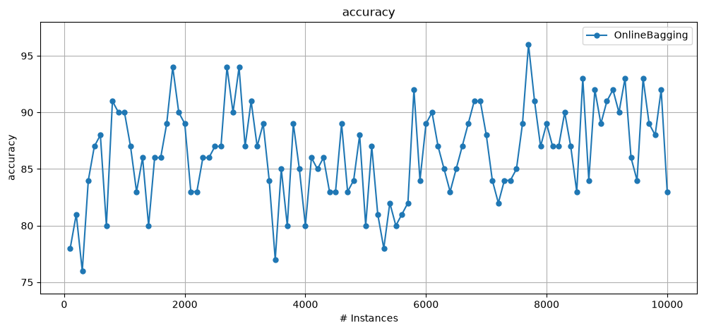
# The drift location is based on the number of instances (5000) as well as the drift width (1000, the default value).
stream_sea1drift = MOAStream(
    moa_stream=ConceptDriftStream(),
    CLI="-s generators.SEAGenerator -d (generators.SEAGenerator -f 2) -p 5000 -w 1000",
)

OB = OnlineBagging(schema=stream_sea1drift.get_schema(), ensemble_size=10)

results_sea1drift_OB = prequential_evaluation(
    stream=stream_sea1drift, learner=OB, window_size=100, max_instances=10000
)

plot_windowed_results(results_sea1drift_OB, metric="accuracy")

The rest of this section is for readers who already know MOA. It shows the same drifting streams built through MOA’s recursive ConceptDriftStream syntax, how a DriftStream behaves when defined from a MOA CLI rather than a list of concepts, and how a recurrent stream looks on the MOA side.

CapyMOA’s own DriftStream API is covered in Simulating concept drifts. It composes concepts in Python, so a concept can be any Stream – including NumpyStream, CSVStream and others MOA cannot represent.

The raw MOA version

• We first show how it is done using MOA’s API, so that one can compare it with CapyMOA syntax.

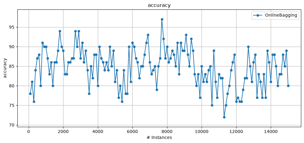
• We simulate the following drifting stream using a traditional recursive MOA syntax:

SEA(function=1), Drift(position=5000, width=1000), SEA(function=2), Drift(position=10000, width=2000), SEA(function=3)

• The CLI below is easy to configure in the MOA GUI, but it can lead to issues when specified directly on the CLI.

from moa.streams import ConceptDriftStream

from capymoa.classifier import OnlineBagging
from capymoa.stream import MOAStream

stream_sea2drift = MOAStream(
    moa_stream=ConceptDriftStream(),
    CLI="-s (ConceptDriftStream -s (generators.SEAGenerator -f 1) -d (generators.SEAGenerator -f 2) -p 5000 -w 1) -d (generators.SEAGenerator -f 3) -p 10000 -w 2000",
)

OB = OnlineBagging(schema=stream_sea2drift.get_schema(), ensemble_size=10)

results_sea2drift_OB = prequential_evaluation(
    stream=stream_sea2drift, learner=OB, window_size=100, max_instances=15000
)

plot_windowed_results(results_sea2drift_OB, metric="accuracy")

Drift metadata from a MOA-defined stream

• Besides composing a drifting stream, the DriftStream object also holds information about the drifts.

• The metadata about the drifts can be used for quickly investigating where and how many Drifts a particular Stream object has associated with it.

• It is doable to extract drifting information from the MOA ConceptDriftStream objects, precisely the Stream objects that form the concepts for a proper printing. However, that has not been implemented yet as it is a bit cumbersome. So, for the moment, when a DriftStream is specified based on a MOA CLI, we just return the CLI used when we attempt to print the object (see below).

print(stream_sea2drift)

• However, the information is available and can be accessed through the get_drifts() method as shown below:

for drift in stream_sea2drift.get_drifts():
    print(f'\t{drift}')

from moa.streams import ConceptDriftStream

from capymoa.stream.drift import DriftStream

stream_sea2drift = DriftStream(
    moa_stream=ConceptDriftStream(),
    CLI="-s (ConceptDriftStream -s generators.SEAGenerator -d (generators.SEAGenerator -f 3) -p 5000 -w 1) \
                                -d generators.SEAGenerator -w 200 -p 10000 -r 1 -a 0.0",
)

OB = OnlineBagging(schema=stream_sea2drift.get_schema(), ensemble_size=10)

results_sea2drift_OB = prequential_evaluation(
    stream=stream_sea2drift, learner=OB, window_size=100, max_instances=12000
)

print(
    f"Attempting to print a stream from a raw MOA ConceptDriftStream: {stream_sea2drift}"
)
print("\nNow, an example on how to access individual drifts from a DriftStream:")
for drift in stream_sea2drift.get_drifts():
    print(f"\t{drift}")
# Notice it works just fine to plot and use the DriftStream created using a MOA object.
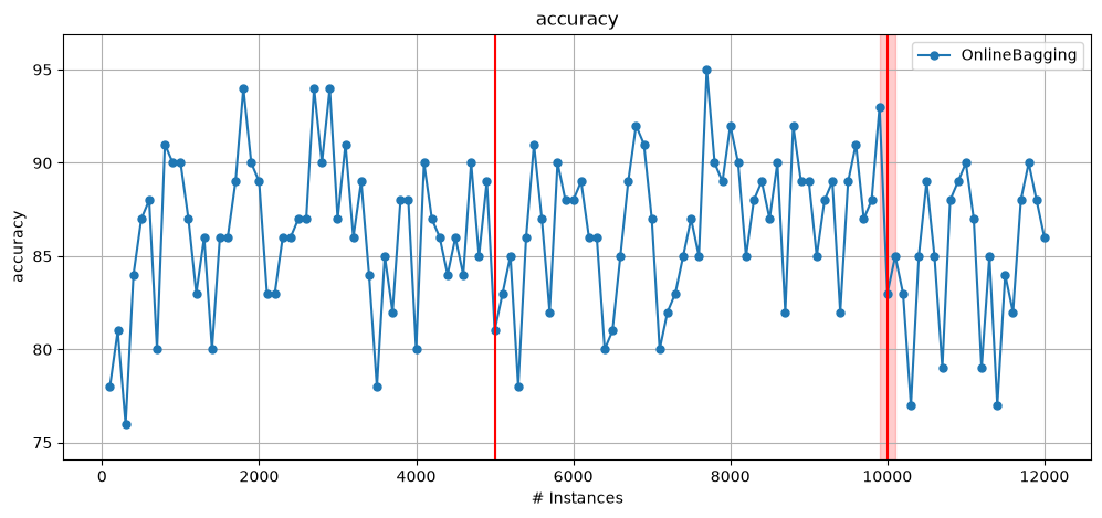
plot_windowed_results(results_sea2drift_OB, metric="accuracy")

Attempting to print a stream from a raw MOA ConceptDriftStream: ConceptDriftStream -s (ConceptDriftStream -s generators.SEAGenerator -d (generators.SEAGenerator -f 3) -p 5000 -w 1)                                 -d generators.SEAGenerator -w 200 -p 10000 -r 1 -a 0.0

Now, an example on how to access individual drifts from a DriftStream:
	AbruptDrift(position=5000)
	GradualDrift(position=10000, width=200)

• A DriftStream composed in Python can be converted the other way with to_moa_stream(), which builds the equivalent nested ConceptDriftStream. That requires every concept to be MOA-backed, and says so when it is not.

A recurrent concept stream as MOA sees it

RecurrentConceptDriftStream cycles through a list of concepts, and the result is an ordinary DriftStream. Printing it shows the concepts and drifts CapyMOA composed; to_moa_stream() shows the same stream as MOA would express it, which grows quickly once concepts recur.

from capymoa.stream.drift import AbruptDrift, RecurrentConceptDriftStream
from capymoa.stream.generator import SEA

stream_with_recurrent_concepts = RecurrentConceptDriftStream(
    concept_list=[SEA(function=1), SEA(function=2), SEA(function=3)],
    max_recurrences_per_concept=2,
    transition_type_template=AbruptDrift(position=2000),
)

print(f"Recurrent concept stream, CapyMOA:\n{stream_with_recurrent_concepts}\n")
print(
    "Recurrent concept stream, MOA CLI:\n"
    f"ConceptDriftStream {stream_with_recurrent_concepts.to_moa_stream()._CLI}"
)

Recurrent concept stream, CapyMOA:
SEA(function=1),AbruptDrift(position=2000),SEA(function=2),AbruptDrift(position=4000),SEA(function=3),AbruptDrift(position=6000),SEA(instance_random_seed=2, function=1),AbruptDrift(position=8000),SEA(instance_random_seed=2, function=2),AbruptDrift(position=10000),SEA(instance_random_seed=2, function=3)

Recurrent concept stream, MOA CLI:
ConceptDriftStream  -s (ConceptDriftStream -s (ConceptDriftStream -s (ConceptDriftStream -s (ConceptDriftStream -s generators.SEAGenerator -d (generators.SEAGenerator -f 2) -p 2000 -w 0) -d (generators.SEAGenerator -f 3) -p 4000 -w 0) -d (generators.SEAGenerator -i 2) -p 6000 -w 0) -d (generators.SEAGenerator -f 2 -i 2) -p 8000 -w 0)  -d (generators.SEAGenerator -f 3 -i 2) -w 0 -p 10000 -r 1

Drift, multi-threaded ensembles and results

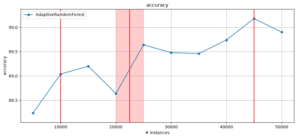
• Generate a stream with 3 drifts: 2 abrupt and one gradual.

• Evaluate utilising test-then-train (cumulative) and windowed evaluation.

• Execute a multi-threaded version of AdaptiveRandomForest.

• For more on multi-threaded ensembles, see the parallel_ensembles.py notebook.

from capymoa.classifier import AdaptiveRandomForestClassifier
from capymoa.evaluation import prequential_evaluation
from capymoa.evaluation.visualization import plot_windowed_results
from capymoa.stream.drift import AbruptDrift, DriftStream, GradualDrift
from capymoa.stream.generator import SEA

SEA3drifts = DriftStream(
    stream=[
        SEA(1),
        AbruptDrift(10000),
        SEA(2),
        GradualDrift(start=20000, end=25000),
        SEA(3),
        AbruptDrift(45000),
        SEA(1),
    ]
)

arf = AdaptiveRandomForestClassifier(
    schema=SEA3drifts.get_schema(), ensemble_size=100, number_of_jobs=4
)

results = prequential_evaluation(
    stream=SEA3drifts, learner=arf, window_size=5000, max_instances=50000
)

print(f"Cumulative accuracy = {results.cumulative.accuracy()}")
print(f"Wallclock = {results.wallclock()} seconds")
display(results.windowed.metrics_per_window())
plot_windowed_results(results, metric="accuracy")

Cumulative accuracy = 89.352
Wallclock = 41.860010385513306 seconds

	instances	accuracy	kappa	kappa_t	kappa_m	f1_score	F1 Score macro (percent)	f1_score_0	f1_score_1	precision	Precision macro (percent)	precision_0	precision_1	recall	Recall macro (percent)	recall_0	recall_1	roc_auc
0	5000.0	88.24	73.655083	74.289462	67.040359	88.24	86.798915	82.437276	91.160553	88.24	88.238718	88.235294	88.242142	88.24	85.816434	77.354260	94.278607	0.858164
1	10000.0	89.04	75.824986	76.867877	70.152505	89.04	87.888023	84.152689	91.623357	89.04	89.212603	89.704069	88.721137	89.04	86.985119	79.248366	94.721871	0.864067
2	15000.0	89.20	76.256806	76.972281	70.715835	89.20	88.106641	84.500574	91.712707	89.20	89.342334	89.756098	88.928571	89.20	87.251635	79.826464	94.676806	0.866913
3	20000.0	88.64	74.836040	75.632776	68.636113	88.64	87.397438	83.440233	91.354642	88.64	88.574308	88.387894	88.760722	88.64	86.560926	79.017118	94.104735	0.866584
4	25000.0	89.64	76.918788	76.988005	71.029083	89.64	88.441576	84.719764	92.163389	89.64	89.639459	89.637953	89.640965	89.64	87.572540	80.313199	94.831880	0.868396
5	30000.0	89.48	76.542090	77.090592	70.532213	89.48	88.252921	84.456265	92.049577	89.48	89.450423	89.368355	89.532490	89.48	87.384154	80.056022	94.712286	0.869295
6	35000.0	89.46	76.149486	76.186173	69.181287	89.46	88.065755	83.986630	92.144880	89.46	88.909791	87.413030	90.406552	89.46	87.385041	80.818713	93.951368	0.869884
7	40000.0	89.74	77.175256	77.647059	71.468298	89.74	88.567888	84.907326	92.228450	89.74	89.843460	90.131168	89.555752	89.74	87.660712	80.255840	95.065584	0.870725
8	45000.0	90.18	78.269005	79.194915	73.051592	90.18	89.113456	85.705968	92.520944	90.18	90.462448	91.258524	89.666371	90.18	88.176794	80.790340	95.563247	0.871957
9	50000.0	89.90	77.510176	77.918671	71.708683	89.90	88.739731	85.125184	92.354277	89.90	89.861027	89.751553	89.970501	89.90	87.910094	80.952381	94.867807	0.872668

AutoML with AutoClass

The following example shows how to use the AutoClass algorithm with CapyMOA.

• AutoClass is configured using a json configuration file settings_autoclass.json and a list of classifiers base_classifiers.

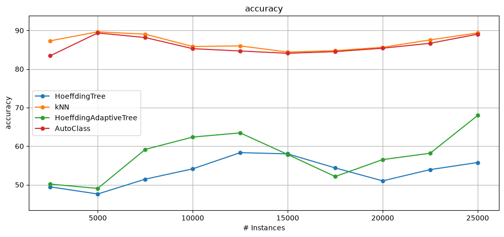
• AutoClass can also be configured with a list of base_classifier strings representing the MOA classifiers. This approach is only enticing for people that are very familiar with MOA.

• In the example below, we also compare it against using the base classifiers individually.

from capymoa.automl import AutoClass
from capymoa.classifier import KNN, HoeffdingAdaptiveTree, HoeffdingTree
from capymoa.datasets import RBFm_100k
from capymoa.evaluation import prequential_evaluation
from capymoa.evaluation.visualization import plot_windowed_results

rbf_100k = RBFm_100k()

max_instances = 25000
window_size = 2500

ht = HoeffdingTree(schema=rbf_100k.get_schema())
hat = HoeffdingAdaptiveTree(schema=rbf_100k.get_schema())
knn = KNN(schema=rbf_100k.get_schema())
autoclass = AutoClass(
    schema=rbf_100k.get_schema(),
    configuration_json="./settings_autoclass.json",
    base_classifiers=[KNN, HoeffdingAdaptiveTree, HoeffdingTree],
)

results_ht = prequential_evaluation(
    stream=rbf_100k, learner=ht, window_size=window_size, max_instances=max_instances
)
results_hat = prequential_evaluation(
    stream=rbf_100k, learner=hat, window_size=window_size, max_instances=max_instances
)
results_knn = prequential_evaluation(
    stream=rbf_100k, learner=knn, window_size=window_size, max_instances=max_instances
)
results_autoclass = prequential_evaluation(
    stream=rbf_100k,
    learner=autoclass,
    window_size=window_size,
    max_instances=max_instances,
)

print(
    f"[HT] Cumulative accuracy = {results_ht.accuracy()}, wall-clock time: {results_ht.wallclock()}"
)
print(
    f"[HAT] Cumulative accuracy = {results_hat.accuracy()}, wall-clock time: {results_hat.wallclock()}"
)
print(
    f"[KNN] Cumulative accuracy = {results_knn.accuracy()}, wall-clock time: {results_knn.wallclock()}"
)
print(
    f"[AUTOCLASS] Cumulative accuracy = {results_autoclass.accuracy()}, wall-clock time: {results_autoclass.wallclock()}"
)
plot_windowed_results(
    results_ht, results_knn, results_hat, results_autoclass, metric="accuracy"
)

[HT] Cumulative accuracy = 53.396, wall-clock time: 0.33103322982788086
[HAT] Cumulative accuracy = 57.676, wall-clock time: 0.3304269313812256
[KNN] Cumulative accuracy = 86.956, wall-clock time: 2.788100004196167
[AUTOCLASS] Cumulative accuracy = 86.064, wall-clock time: 74.61233973503113

AutoClass alternative syntax

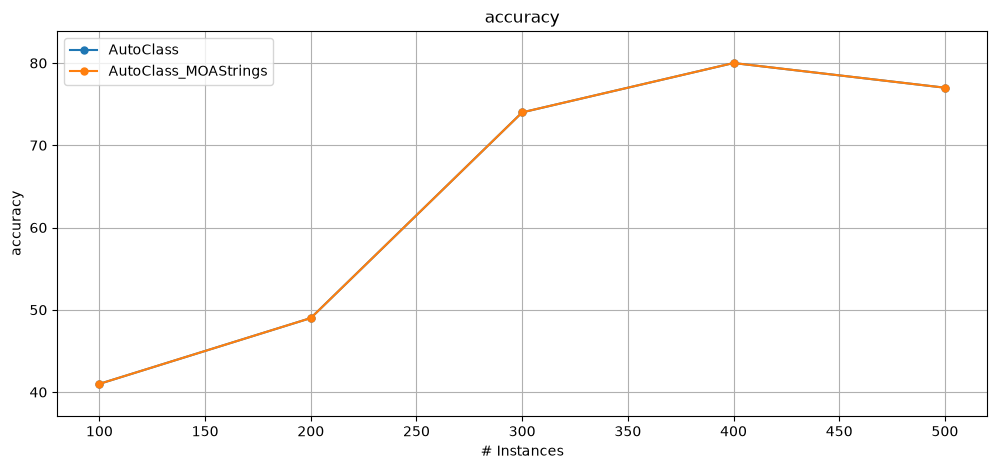
Another way to configure the learners is by using a list of string base_classifiers representing the MOA classifiers.

from capymoa.automl import AutoClass
from capymoa.classifier import KNN, HoeffdingAdaptiveTree, HoeffdingTree, OnlineBagging
from capymoa.datasets import RBFm_100k
from capymoa.evaluation import prequential_evaluation
from capymoa.evaluation.visualization import plot_windowed_results

rbf_100k = RBFm_100k()

autoclass = AutoClass(
    schema=rbf_100k.get_schema(),
    configuration_json="./settings_autoclass.json",
    base_classifiers=[KNN, HoeffdingTree, HoeffdingAdaptiveTree],
)

autoclass_MOAStrings = AutoClass(
    schema=rbf_100k.get_schema(),
    configuration_json="./settings_autoclass.json",
    base_classifiers=["lazy.kNN", "trees.HoeffdingTree", "trees.HoeffdingAdaptiveTree"],
)

results_autoClass = prequential_evaluation(
    stream=rbf_100k, learner=autoclass, window_size=100, max_instances=500
)
results_autoclass_MOAStrings = prequential_evaluation(
    stream=rbf_100k, learner=autoclass_MOAStrings, window_size=100, max_instances=500
)

results_autoclass_MOAStrings.learner = "AutoClass_MOAStrings"

plot_windowed_results(
    results_autoClass, results_autoclass_MOAStrings, metric="accuracy"
)