Semi-supervised Learning

• Preparing and executing partially and delayed labeling experiments.

---

More information about CapyMOA can be found at https://www.capymoa.org.

last update on 01/12/2025

from capymoa.evaluation.visualization import plot_windowed_results
from capymoa.evaluation import prequential_ssl_evaluation
from capymoa.datasets import Electricity

1. Learning using a SSL classifier

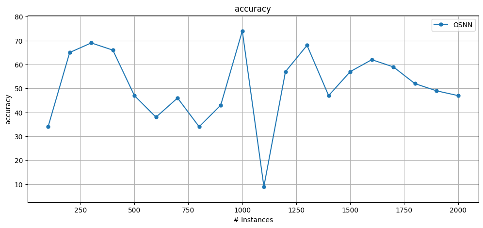
• This example uses the OSNN algorithm to learn from a stream with only 1% labeled data.

• We utilise the prequential_ssl_evaluation() function to simulate the absence of labels (label_probability) and delays (delay_length).

• The results yielded by prequential_ssl_evaluation() include more information in comparison to prequential_evaluation(), such as the number of unlabeled instances (unlabeled) and the unlabeled ratio (unlabeled_ratio).

help(prequential_ssl_evaluation)

Help on function prequential_ssl_evaluation in module capymoa.evaluation.evaluation:

prequential_ssl_evaluation(
    stream: capymoa.stream._stream.Stream,
    learner: Union[capymoa.base._ssl.ClassifierSSL, capymoa.base._classifier.Classifier],
    max_instances: Optional[int] = None,
    window_size: int = 1000,
    initial_window_size: int = 0,
    delay_length: int = 0,
    label_probability: float = 0.01,
    random_seed: int = 1,
    store_predictions: bool = False,
    store_y: bool = False,
    optimise: bool = True,
    restart_stream: bool = True,
    progress_bar: Union[bool, tqdm.std.tqdm] = False,
    batch_size: int = 1
)
    Run and evaluate a learner on a semi-supervised stream using prequential evaluation.

    :param stream: A data stream to evaluate the learner on. Will be restarted if
        ``restart_stream`` is True.
    :param learner: The learner to evaluate. If the learner is an SSL learner,
        it will be trained on both labeled and unlabeled instances. If the
        learner is not an SSL learner, then it will be trained only on the
        labeled instances.
    :param max_instances: The number of instances to evaluate before exiting.
        If None, the evaluation will continue until the stream is empty.
    :param window_size: The size of the window used for windowed evaluation,
        defaults to 1000
    :param initial_window_size: Not implemented yet
    :param delay_length: If greater than zero the labeled (``label_probability``%)
        instances will appear as unlabeled before reappearing as labeled after
        ``delay_length`` instances, defaults to 0
    :param label_probability: The proportion of instances that will be labeled,
        must be in the range [0, 1], defaults to 0.01
    :param random_seed: A random seed to define the random state that decides
        which instances are labeled and which are not, defaults to 1.
    :param store_predictions: Store the learner's prediction in a list, defaults
        to False
    :param store_y: Store the ground truth targets in a list, defaults to False
    :param optimise: If True and the learner is compatible, the evaluator will
        use a Java native evaluation loop, defaults to True.
    :param restart_stream: If False, evaluation will continue from the current
        position in the stream, defaults to True. Not restarting the stream is
        useful for switching between learners or evaluators, without starting
        from the beginning of the stream.
    :param progress_bar: Enable, disable, or override the progress bar. Currently
        incompatible with ``optimize=True``.
    :return: An object containing the results of the evaluation windowed metrics,
        cumulative metrics, ground truth targets, and predictions.

from capymoa.ssl import OSNN

stream = Electricity()

osnn = OSNN(schema=stream.get_schema(), optim_steps=10)

results_osnn = prequential_ssl_evaluation(
    stream=stream,
    learner=osnn,
    label_probability=0.01,
    window_size=100,
    max_instances=2000,
)

# The results are stored in a dictionary.
display(results_osnn)

print(
    results_osnn["cumulative"].accuracy()
)  # Test-then-train accuracy, i.e. cumulatively, not windowed.

# Plotting over time (default: classifications correct (percent) i.e. accuracy)
results_osnn.learner = "OSNN"
plot_windowed_results(results_osnn, metric="accuracy")

<capymoa.evaluation.results.PrequentialResults at 0x75269353d160>

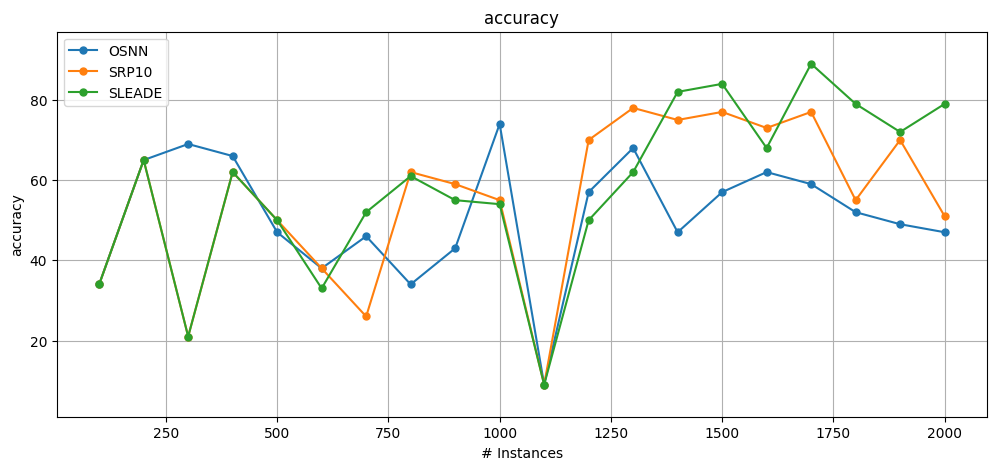
51.15

1.1 Using a supervised model

• If a supervised model is used with prequential_ssl_evaluation(), it will only be trained on the labeled data.

from capymoa.classifier import StreamingRandomPatches

srp10 = StreamingRandomPatches(schema=stream.get_schema(), ensemble_size=10)

results_srp10 = prequential_ssl_evaluation(
    stream=stream,
    learner=srp10,
    label_probability=0.01,
    window_size=100,
    max_instances=2000,
)
print(results_srp10["cumulative"].accuracy())

55.35

1.2 SLEADE

• SLEADE is another semi-supervised learning algorithm

from capymoa.ssl import SLEADE

stream = Electricity()

sleade = SLEADE(
    schema=stream.get_schema(), base_ensemble="StreamingRandomPatches -s 10"
)

results_sleade = prequential_ssl_evaluation(
    stream=stream,
    learner=sleade,
    label_probability=0.01,
    window_size=100,
    max_instances=2000,
)

print(results_sleade["cumulative"].accuracy())

58.050000000000004

1.3 Comparing a SSL classifier to a supervised classifier

# Plotting all the results together
# Adding an experiment_id to the results dictionary allows controlling the legend of each learner.
results_osnn.learner = "OSNN"
results_srp10.learner = "SRP10"
results_sleade.learner = "SLEADE"

plot_windowed_results(results_osnn, results_srp10, results_sleade, metric="accuracy")

2. Delay example

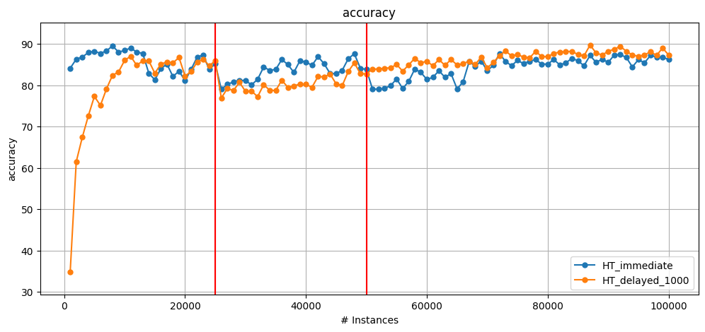
• In this section we compare the effect of delay on a stream.

• It is particularly interesting to see the effect after a drift takes place.

from capymoa.stream.generator import SEA
from capymoa.stream.drift import DriftStream, AbruptDrift
from capymoa.classifier import HoeffdingTree

## Creating a stream with drift
sea2drifts = DriftStream(
    stream=[
        SEA(function=1),
        AbruptDrift(position=25000),
        SEA(function=2),
        AbruptDrift(position=50000),
        SEA(function=3),
    ]
)


ht_immediate = HoeffdingTree(schema=sea2drifts.get_schema())
ht_delayed = HoeffdingTree(schema=sea2drifts.get_schema())

results_ht_immediate = prequential_ssl_evaluation(
    stream=sea2drifts,
    learner=ht_immediate,
    label_probability=0.1,
    window_size=1000,
    max_instances=100000,
)

results_ht_delayed_1000 = prequential_ssl_evaluation(
    stream=sea2drifts,
    learner=ht_delayed,
    label_probability=0.01,
    delay_length=1000,  # adding the delay
    window_size=1000,
    max_instances=100000,
)

results_ht_immediate.learner = "HT_immediate"
results_ht_delayed_1000.learner = "HT_delayed_1000"

print(f"Accuracy immediate: {results_ht_immediate['cumulative'].accuracy()}")
print(
    f"Accuracy delayed by 1000 instances: {results_ht_delayed_1000['cumulative'].accuracy()}"
)

plot_windowed_results(results_ht_immediate, results_ht_delayed_1000, metric="accuracy")

Accuracy immediate: 84.517
Accuracy delayed by 1000 instances: 83.366